#############################################
import pandas as pd
import numpy as np
import statsmodels.formula.api as smf
import matplotlib.pyplot as plt
#############################################
문제1. Linear Regression (총 30점)
a. 주어진 데이터를 데이터프레임화 하기 (DataFrame) (5점)
b. 데이터를 바탕으로 선형회귀식을 구하시오. (5점) 이때, CRIM, NDUS, NOX, AGE, PTRATIO 를 독립변수로 활용하시오.
c. 유의수준 0.05에서 유의미하다고 판단되는 독립변수를 찾고, 해당 변수의 회귀계수의 의미를 해석하시오. (10점)
d. 결과들을 바탕으로 결정계수를 구하고 그 의미를 종속변수의 총변동(SST)를 활용하여 설명할 것. (10점)
보스턴 주택가격 데이터
종속변수
- PRICE: 본인 소유의 주택 가격 (단위: 달러)
독립변수
- CRIM: 지역별 범죄 발생률 (단위: %)
- ZN: 25,000평방피트를 초과하는 거주 지역의 비율
- NDUS: 비상업 지역 넓이 비율 (단위: %)
- CHAS: 찰스강에 대한 더미 변수(강의 경계에 위치한 경우는 1, 아니면 0)
- NOX: 일산화질소 농도 (단위: ppm)
- RM: 거주할 수 있는 방 개수
- AGE: 1940년 이전에 건축된 소유 주택의 비율 (단위: %)
- DIS: 5개 주요 고용센터까지의 가중 거리
- RAD: 고속도로 접근 용이도
- TAX: 10,000달러당 재산세율
- PTRATIO: 지역의 교사대비 학생 수 비율 (단위: %)
- LSTAT: 하위 계층의 비율
#######이 셀을 실행하면 데이터가 받아집니다. 실행만 하고 이 셀을 변형시키려 하지 마세요.###########
import pandas as pd
import numpy as np
data_url = "http://lib.stat.cmu.edu/datasets/boston"
raw_df = pd.read_csv(data_url, sep="\s+", skiprows=22, header=None)
data = np.hstack([raw_df.values[::2, :], raw_df.values[1::2, :2]])
data = np.delete(data, 11, axis = 1) #독립변수 데이터
target = raw_df.values[1::2, 2] #종속변수 데이터print('data: ', data)
print('target: ', target)data: [[6.3200e-03 1.8000e+01 2.3100e+00 ... 2.9600e+02 1.5300e+01 4.9800e+00]
[2.7310e-02 0.0000e+00 7.0700e+00 ... 2.4200e+02 1.7800e+01 9.1400e+00]
[2.7290e-02 0.0000e+00 7.0700e+00 ... 2.4200e+02 1.7800e+01 4.0300e+00]
...
[6.0760e-02 0.0000e+00 1.1930e+01 ... 2.7300e+02 2.1000e+01 5.6400e+00]
[1.0959e-01 0.0000e+00 1.1930e+01 ... 2.7300e+02 2.1000e+01 6.4800e+00]
[4.7410e-02 0.0000e+00 1.1930e+01 ... 2.7300e+02 2.1000e+01 7.8800e+00]]
target: [24. 21.6 34.7 33.4 36.2 28.7 22.9 27.1 16.5 18.9 15. 18.9 21.7 20.4
18.2 19.9 23.1 17.5 20.2 18.2 13.6 19.6 15.2 14.5 15.6 13.9 16.6 14.8
18.4 21. 12.7 14.5 13.2 13.1 13.5 18.9 20. 21. 24.7 30.8 34.9 26.6
25.3 24.7 21.2 19.3 20. 16.6 14.4 19.4 19.7 20.5 25. 23.4 18.9 35.4
24.7 31.6 23.3 19.6 18.7 16. 22.2 25. 33. 23.5 19.4 22. 17.4 20.9
24.2 21.7 22.8 23.4 24.1 21.4 20. 20.8 21.2 20.3 28. 23.9 24.8 22.9
23.9 26.6 22.5 22.2 23.6 28.7 22.6 22. 22.9 25. 20.6 28.4 21.4 38.7
43.8 33.2 27.5 26.5 18.6 19.3 20.1 19.5 19.5 20.4 19.8 19.4 21.7 22.8
18.8 18.7 18.5 18.3 21.2 19.2 20.4 19.3 22. 20.3 20.5 17.3 18.8 21.4
15.7 16.2 18. 14.3 19.2 19.6 23. 18.4 15.6 18.1 17.4 17.1 13.3 17.8
14. 14.4 13.4 15.6 11.8 13.8 15.6 14.6 17.8 15.4 21.5 19.6 15.3 19.4
17. 15.6 13.1 41.3 24.3 23.3 27. 50. 50. 50. 22.7 25. 50. 23.8
23.8 22.3 17.4 19.1 23.1 23.6 22.6 29.4 23.2 24.6 29.9 37.2 39.8 36.2
37.9 32.5 26.4 29.6 50. 32. 29.8 34.9 37. 30.5 36.4 31.1 29.1 50.
33.3 30.3 34.6 34.9 32.9 24.1 42.3 48.5 50. 22.6 24.4 22.5 24.4 20.
21.7 19.3 22.4 28.1 23.7 25. 23.3 28.7 21.5 23. 26.7 21.7 27.5 30.1
44.8 50. 37.6 31.6 46.7 31.5 24.3 31.7 41.7 48.3 29. 24. 25.1 31.5
23.7 23.3 22. 20.1 22.2 23.7 17.6 18.5 24.3 20.5 24.5 26.2 24.4 24.8
29.6 42.8 21.9 20.9 44. 50. 36. 30.1 33.8 43.1 48.8 31. 36.5 22.8
30.7 50. 43.5 20.7 21.1 25.2 24.4 35.2 32.4 32. 33.2 33.1 29.1 35.1
45.4 35.4 46. 50. 32.2 22. 20.1 23.2 22.3 24.8 28.5 37.3 27.9 23.9
21.7 28.6 27.1 20.3 22.5 29. 24.8 22. 26.4 33.1 36.1 28.4 33.4 28.2
22.8 20.3 16.1 22.1 19.4 21.6 23.8 16.2 17.8 19.8 23.1 21. 23.8 23.1
20.4 18.5 25. 24.6 23. 22.2 19.3 22.6 19.8 17.1 19.4 22.2 20.7 21.1
19.5 18.5 20.6 19. 18.7 32.7 16.5 23.9 31.2 17.5 17.2 23.1 24.5 26.6
22.9 24.1 18.6 30.1 18.2 20.6 17.8 21.7 22.7 22.6 25. 19.9 20.8 16.8
21.9 27.5 21.9 23.1 50. 50. 50. 50. 50. 13.8 13.8 15. 13.9 13.3
13.1 10.2 10.4 10.9 11.3 12.3 8.8 7.2 10.5 7.4 10.2 11.5 15.1 23.2
9.7 13.8 12.7 13.1 12.5 8.5 5. 6.3 5.6 7.2 12.1 8.3 8.5 5.
11.9 27.9 17.2 27.5 15. 17.2 17.9 16.3 7. 7.2 7.5 10.4 8.8 8.4
16.7 14.2 20.8 13.4 11.7 8.3 10.2 10.9 11. 9.5 14.5 14.1 16.1 14.3
11.7 13.4 9.6 8.7 8.4 12.8 10.5 17.1 18.4 15.4 10.8 11.8 14.9 12.6
14.1 13. 13.4 15.2 16.1 17.8 14.9 14.1 12.7 13.5 14.9 20. 16.4 17.7
19.5 20.2 21.4 19.9 19. 19.1 19.1 20.1 19.9 19.6 23.2 29.8 13.8 13.3
16.7 12. 14.6 21.4 23. 23.7 25. 21.8 20.6 21.2 19.1 20.6 15.2 7.
8.1 13.6 20.1 21.8 24.5 23.1 19.7 18.3 21.2 17.5 16.8 22.4 20.6 23.9
22. 11.9]a. 주어진 데이터를 테이터프레임화 하기. (5점)
# data 변수는 아래 컬럼명 순서대로 열이 배치되어 있음.

columns_name = ['CRIM', 'ZN', 'NDUS', 'CHAS', 'NOX', 'RM', 'AGE', 'DIS', 'RAD', 'TAX', 'PTRATIO', 'LSTAT']
# data = 독립변수 데이터
# target = 종속변수 데이터
#############################################
X_df = pd.DataFrame(data = data, columns = columns_name)
X_df = X_df[['CRIM', 'NDUS', 'NOX', 'AGE', 'PTRATIO']]
y_df = pd.DataFrame(data = target, columns = ['price'])
df = pd.concat([X_df, y_df], axis = 1)
df
#############################################| CRIM | NDUS | NOX | AGE | PTRATIO | price | |
|---|---|---|---|---|---|---|
| 0 | 0.00632 | 2.31 | 0.538 | 65.2 | 15.3 | 24.0 |
| 1 | 0.02731 | 7.07 | 0.469 | 78.9 | 17.8 | 21.6 |
| 2 | 0.02729 | 7.07 | 0.469 | 61.1 | 17.8 | 34.7 |
| 3 | 0.03237 | 2.18 | 0.458 | 45.8 | 18.7 | 33.4 |
| 4 | 0.06905 | 2.18 | 0.458 | 54.2 | 18.7 | 36.2 |
| ... | ... | ... | ... | ... | ... | ... |
| 501 | 0.06263 | 11.93 | 0.573 | 69.1 | 21.0 | 22.4 |
| 502 | 0.04527 | 11.93 | 0.573 | 76.7 | 21.0 | 20.6 |
| 503 | 0.06076 | 11.93 | 0.573 | 91.0 | 21.0 | 23.9 |
| 504 | 0.10959 | 11.93 | 0.573 | 89.3 | 21.0 | 22.0 |
| 505 | 0.04741 | 11.93 | 0.573 | 80.8 | 21.0 | 11.9 |
506 rows × 6 columns
<svg xmlns="http://www.w3.org/2000/svg" height="24px"viewBox="0 0 24 24"
width="24px">
b. 데이터를 바탕으로 선형회귀식을 구하시오. (5점)
- 이때, 독립변수: CRIM, NDUS, NOX, AGE, PTRATIO /종속변수: PRICE
#############################################
model = smf.ols('price ~ CRIM + NDUS + NOX + AGE + PTRATIO', data = df).fit()
model.summary()
#############################################| Dep. Variable: | price | R-squared: | 0.395 |
|---|---|---|---|
| Model: | OLS | Adj. R-squared: | 0.389 |
| Method: | Least Squares | F-statistic: | 65.27 |
| Date: | Sun, 18 Jun 2023 | Prob (F-statistic): | 2.12e-52 |
| Time: | 12:45:42 | Log-Likelihood: | -1713.1 |
| No. Observations: | 506 | AIC: | 3438. |
| Df Residuals: | 500 | BIC: | 3464. |
| Df Model: | 5 | ||
| Covariance Type: | nonrobust |
| coef | std err | t | P>|t| | [0.025 | 0.975] | |
|---|---|---|---|---|---|---|
| Intercept | 63.3828 | 3.816 | 16.608 | 0.000 | 55.885 | 70.881 |
| CRIM | -0.1527 | 0.042 | -3.609 | 0.000 | -0.236 | -0.070 |
| NDUS | -0.1757 | 0.079 | -2.228 | 0.026 | -0.331 | -0.021 |
| NOX | -15.5243 | 5.086 | -3.052 | 0.002 | -25.517 | -5.532 |
| AGE | 5.59e-05 | 0.017 | 0.003 | 0.997 | -0.034 | 0.034 |
| PTRATIO | -1.6111 | 0.167 | -9.655 | 0.000 | -1.939 | -1.283 |
| Omnibus: | 195.283 | Durbin-Watson: | 0.849 |
|---|---|---|---|
| Prob(Omnibus): | 0.000 | Jarque-Bera (JB): | 744.372 |
| Skew: | 1.755 | Prob(JB): | 2.30e-162 |
| Kurtosis: | 7.794 | Cond. No. | 1.41e+03 |
Notes:
[1] Standard Errors assume that the covariance matrix of the errors is correctly specified.
[2] The condition number is large, 1.41e+03. This might indicate that there are
strong multicollinearity or other numerical problems.
정답
a.
b. CRIM, NDUS, NOX, PTRATIO
- CRIM: 지역별 범죄 발생율이 1% 증가하면 주택가격은 0.1527 달러 감소한다.
- NDUS: 비상업지역 넓이 비율이 1% 증가하면 주택가격은 0.1757 달러 감소한다.
- NOX: 일산화질소 농도가 1ppm 증가하면 주택가격은 15.5243 달러 감소한다.
- PTRATIO: 지역의 교사대비 학생수 비율이 1% 증가하면 주택가격은 1.6111 달러 감소한다.
c. 0.395, 결정계수는 총변동(SST)에서 회귀제곱값 SSR이 차지하는 비율이다. 즉, y의 총변동중 선형회귀모형에 의하여 39.5%만큼 설명될 수 있다.
문제2. Logistic Regression (총 30점)
a. 주어진 데이터를 데이터프레임화 하기 (DataFrame) (10점)
b. 데이터를 바탕으로 로지스틱 회귀식을 구하시오. (5점) 이때, 독립변수는 mean radius 만 사용할 것.
c. 실제 데이터와 로지스틱 회귀식을 한 그림에 겹쳐서 그릴 것. (5점)
d. 독립변수의 회귀계수의 의미를 로짓변환의 관점에서 해석할 것. (5점)
e. 독립변수의 승산비율을 구하고 의미를 해석할 것. (5점)
유방암 진단 데이터
종속변수
- cancer : 암에 걸리면 0, 아니면 1
독립변수 (사진으로 찍은 종양의 특징들)
- mean_radius: 종양의 반지름 (단위: mm)
- mean_texture: 종양 질감
- mean_perimeter: 종양 둘레
- mean_area: 종양 면적
- mean_smoothness: 종양 매끄러움 정도
- mean_compactness: 종양의 조그만 정도
- mean_concavity: 종양의 오목함 정도
- mean_concave points: 종양의 오목한 점의 수
- mean_symmetry: 종양의 대칭 정도
- mean_fractal dimension: 종양의 프랙탈 차원
#######이 셀을 실행하면 데이터가 받아집니다. 실행만 하고 이 셀을 변형시키려 하지 마세요.###########
import pandas as pd
import numpy as np
from sklearn.datasets import load_breast_cancer

breast_cancer = load_breast_cancer()
data = breast_cancer.data[:, :10] #독립변수
target = breast_cancer.target #종속변수
print(data.shape)
print(target.shape)
(569, 10)
(569,)# data 변수는 아래 컬럼명 순서대로 열이 배치되어 있음.
columns_name = breast_cancer.feature_names[:10]
print(columns_name)['mean radius' 'mean texture' 'mean perimeter' 'mean area'
'mean smoothness' 'mean compactness' 'mean concavity'
'mean concave points' 'mean symmetry' 'mean fractal dimension']a. 주어진 데이터를 테이터프레임화 하기. (10점)
-
이때, 종속변수가 0과 1로 구성되어 있는데, 0이었던 값은 1로, 1이었던 값은 0으로 바꿔서 데이터프레임화할 것. (양성이 0, 음성이 1 이었던 것을 음성이 0, 양성이 1이 되도록)
-
컬럼명 사이에 띄어쓰기가 되어 있는데 (ex, mean radius) 띄어쓰기를 없애고 underbar 로 대체할 것. (ex, mean_radius)
#############################################
columns_name = [col.replace(' ', '_') for col in columns_name] #변별력
X_df = pd.DataFrame(data = data, columns = columns_name)
y_df = pd.DataFrame(data = target, columns = ['label'])
df = pd.concat([X_df, y_df], axis = 1)
df['label'] = df['label'].replace([0, 1], [1, 0])
df
#############################################| mean_radius | mean_texture | mean_perimeter | mean_area | mean_smoothness | mean_compactness | mean_concavity | mean_concave_points | mean_symmetry | mean_fractal_dimension | label | |
|---|---|---|---|---|---|---|---|---|---|---|---|
| 0 | 17.99 | 10.38 | 122.80 | 1001.0 | 0.11840 | 0.27760 | 0.30010 | 0.14710 | 0.2419 | 0.07871 | 1 |
| 1 | 20.57 | 17.77 | 132.90 | 1326.0 | 0.08474 | 0.07864 | 0.08690 | 0.07017 | 0.1812 | 0.05667 | 1 |
| 2 | 19.69 | 21.25 | 130.00 | 1203.0 | 0.10960 | 0.15990 | 0.19740 | 0.12790 | 0.2069 | 0.05999 | 1 |
| 3 | 11.42 | 20.38 | 77.58 | 386.1 | 0.14250 | 0.28390 | 0.24140 | 0.10520 | 0.2597 | 0.09744 | 1 |
| 4 | 20.29 | 14.34 | 135.10 | 1297.0 | 0.10030 | 0.13280 | 0.19800 | 0.10430 | 0.1809 | 0.05883 | 1 |
| ... | ... | ... | ... | ... | ... | ... | ... | ... | ... | ... | ... |
| 564 | 21.56 | 22.39 | 142.00 | 1479.0 | 0.11100 | 0.11590 | 0.24390 | 0.13890 | 0.1726 | 0.05623 | 1 |
| 565 | 20.13 | 28.25 | 131.20 | 1261.0 | 0.09780 | 0.10340 | 0.14400 | 0.09791 | 0.1752 | 0.05533 | 1 |
| 566 | 16.60 | 28.08 | 108.30 | 858.1 | 0.08455 | 0.10230 | 0.09251 | 0.05302 | 0.1590 | 0.05648 | 1 |
| 567 | 20.60 | 29.33 | 140.10 | 1265.0 | 0.11780 | 0.27700 | 0.35140 | 0.15200 | 0.2397 | 0.07016 | 1 |
| 568 | 7.76 | 24.54 | 47.92 | 181.0 | 0.05263 | 0.04362 | 0.00000 | 0.00000 | 0.1587 | 0.05884 | 0 |
569 rows × 11 columns
<svg xmlns="http://www.w3.org/2000/svg" height="24px"viewBox="0 0 24 24"
width="24px">
b. 데이터를 바탕으로 로지스틱 회귀식을 구하시오.
- 이때, 독립변수: mean_radius
#############################################
model = smf.logit('label ~ mean_radius', data = df).fit()
model.summary()
#############################################
Optimization terminated successfully.
Current function value: 0.289992
Iterations 8| Dep. Variable: | label | No. Observations: | 569 |
|---|---|---|---|
| Model: | Logit | Df Residuals: | 567 |
| Method: | MLE | Df Model: | 1 |
| Date: | Sun, 18 Jun 2023 | Pseudo R-squ.: | 0.5608 |
| Time: | 14:28:43 | Log-Likelihood: | -165.01 |
| converged: | True | LL-Null: | -375.72 |
| Covariance Type: | nonrobust | LLR p-value: | 1.192e-93 |
| coef | std err | z | P>|z| | [0.025 | 0.975] | |
|---|---|---|---|---|---|---|
| Intercept | -15.2459 | 1.325 | -11.509 | 0.000 | -17.842 | -12.649 |
| mean_radius | 1.0336 | 0.093 | 11.100 | 0.000 | 0.851 | 1.216 |
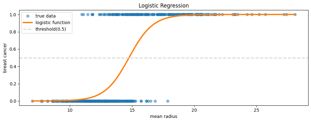
c. 실제 데이터와 로지스틱 회귀선을 한 그림에 겹쳐서 그릴 것.
plt.figure(figsize=(10, 4))

####################################################################
sorted_x = df['mean_radius'].sort_values() #데이터 시각화를 위한 x값 오름차순 정렬
y = 1/(1+np.exp(15.2459 - 1.0336 * sorted_x)) # 데이터 x를 우리가 구한 로지스틱함수를 통해 y 값구하기
plt.plot(df['mean_radius'], df['label'], 'o', alpha = 0.5, label = 'true data') #실제 데이터
plt.plot(sorted_x, y, label = 'logistic function', linewidth = 3) #우리가 추측한 로지스틱 함수
plt.axhline(0.5, color='lightgray', linestyle='--', linewidth=2, label = 'threshold(0.5)')
plt.title('Logistic Regression')
plt.legend()
plt.xlabel('mean radius')
plt.ylabel('breast cancer')
plt.tight_layout()
####################################################################
정답
a.
b. Logit = -15.2459 + 1.0336x_{radius} -> 종양의 반지름이 1mm 증가하면 암에 걸릴 확률의 로짓값이 1.0336 증가한다.
c. Odds Ratio: 2.811 -> 종양의 반지름이 1mm 증가하면 암에 걸릴 확률의 오즈가 2.811배 증가한다.
문제3. Poisson / Negative Binomial Regression (35점)
a. 주어진 데이터를 데이터프레임화 하기 (DataFrame) (10점)
b. 푸아송 회귀모델과 음이항 회귀모델 중 어떤 모델을 선택할 것인지 이유와 함께 제시하라.
    - 이때, 알파값에 대한 가설검정의 유의수준은 0.05로하며, 독립변수는 High Temp (°F) 와 Precipitation 만 사용할 것.(10점)
c. 데이터를 바탕으로 선택한 회귀모델의 회귀식을 구하시오. High Temp (°F) 와 Precipitation(5점)
d. 유의수준 0.05에서 유의미하다고 판단되는 독립변수를 찾고, 해당 변수의 IRR(Incidence Rate Ratio)을 구하고, 의미를 해석하시오. (10점)
날씨에 따른 하루동안 다리(bridge)를 지나가는 자전거 수 데이터
종속변수
- Manhattan Bridge: 하루동안 맨하튼 다리를 건너는 자전거 수
독립변수
- Date: 날짜
- Day: 날짜
- High Temp (°F) : 최고온도 (단위: 도)
- Low Temp (°F): 최저온도
- Precipitation: 강수량 (단위: mm)
- Brooklyn Bridge: 하루동안 브루클린 다리를 건너는 자전거 수
- Williamsburg Bridge: 하루동안 윌리엄스버그 다리를 건너는 자전거 수
- Queensboro Bridge: 하루동안 퀸스보로 다리를 건너는 자전거 수
#######이 셀을 실행하면 데이터가 받아집니다. 실행만 하고 이 셀을 변형시키려 하지 마세요.###########
df = pd.read_csv('https://raw.githubusercontent.com/ericoh929/Machine-Learning/main/nyc-east-river-bicycle-counts.csv')
df.drop(['Total'], axis = 1, inplace = True)
df.replace({'Precipitation':'0.47 (S)'}, 0.47, inplace = True)
df.replace({'Precipitation':'T'}, 0, inplace = True)
df| Unnamed: 0 | Date | Day | High Temp (°F) | Low Temp (°F) | Precipitation | Brooklyn Bridge | Manhattan Bridge | Williamsburg Bridge | Queensboro Bridge | |
|---|---|---|---|---|---|---|---|---|---|---|
| 0 | 0 | 2016-04-01 00:00:00 | 2016-04-01 00:00:00 | 78.1 | 66.0 | 0.01 | 1704.0 | 3126 | 4115.0 | 2552.0 |
| 1 | 1 | 2016-04-02 00:00:00 | 2016-04-02 00:00:00 | 55.0 | 48.9 | 0.15 | 827.0 | 1646 | 2565.0 | 1884.0 |
| 2 | 2 | 2016-04-03 00:00:00 | 2016-04-03 00:00:00 | 39.9 | 34.0 | 0.09 | 526.0 | 1232 | 1695.0 | 1306.0 |
| 3 | 3 | 2016-04-04 00:00:00 | 2016-04-04 00:00:00 | 44.1 | 33.1 | 0.47 | 521.0 | 1067 | 1440.0 | 1307.0 |
| 4 | 4 | 2016-04-05 00:00:00 | 2016-04-05 00:00:00 | 42.1 | 26.1 | 0 | 1416.0 | 2617 | 3081.0 | 2357.0 |
| ... | ... | ... | ... | ... | ... | ... | ... | ... | ... | ... |
| 205 | 205 | 2016-04-26 00:00:00 | 2016-04-26 00:00:00 | 60.1 | 46.9 | 0.24 | 1997.0 | 3520 | 4559.0 | 2929.0 |
| 206 | 206 | 2016-04-27 00:00:00 | 2016-04-27 00:00:00 | 62.1 | 46.9 | 0 | 3343.0 | 5606 | 6577.0 | 4388.0 |
| 207 | 207 | 2016-04-28 00:00:00 | 2016-04-28 00:00:00 | 57.9 | 48.0 | 0 | 2486.0 | 4152 | 5336.0 | 3657.0 |
| 208 | 208 | 2016-04-29 00:00:00 | 2016-04-29 00:00:00 | 57.0 | 46.9 | 0.05 | 2375.0 | 4178 | 5053.0 | 3348.0 |
| 209 | 209 | 2016-04-30 00:00:00 | 2016-04-30 00:00:00 | 64.0 | 48.0 | 0 | 3199.0 | 4952 | 5675.0 | 3606.0 |
210 rows × 10 columns
<svg xmlns="http://www.w3.org/2000/svg" height="24px"viewBox="0 0 24 24"
width="24px">
a. 주어진 데이터를 테이터프레임화 하기. (10점)
- 컬럼명 사이에 띄어쓰기가 되어 있는데 (ex, Brooklyn Bridge) 띄어쓰기를 없애고 underbar 로 대체할 것. (ex, Brooklyn_Bridge)
- 컬럼명에 있는 화씨 표시를 없앨 것 (°F)
- Precipitation 컬럼이 문자열 타입으로 되어 있는데, 실수형 타입으로 바꿀 것.
#################################################################
df.columns = [col.replace(' ', '_') for col in df.columns]
df.rename(columns = {'High_Temp_(°F)': 'High_Temp', 'Low_Temp_(°F)': 'Low_Temp'}, inplace = True)
df = df.astype({'Precipitation':'float'})
df
#################################################################| Unnamed:_0 | Date | Day | High_Temp | Low_Temp | Precipitation | Brooklyn_Bridge | Manhattan_Bridge | Williamsburg_Bridge | Queensboro_Bridge | |
|---|---|---|---|---|---|---|---|---|---|---|
| 0 | 0 | 2016-04-01 00:00:00 | 2016-04-01 00:00:00 | 78.1 | 66.0 | 0.01 | 1704.0 | 3126 | 4115.0 | 2552.0 |
| 1 | 1 | 2016-04-02 00:00:00 | 2016-04-02 00:00:00 | 55.0 | 48.9 | 0.15 | 827.0 | 1646 | 2565.0 | 1884.0 |
| 2 | 2 | 2016-04-03 00:00:00 | 2016-04-03 00:00:00 | 39.9 | 34.0 | 0.09 | 526.0 | 1232 | 1695.0 | 1306.0 |
| 3 | 3 | 2016-04-04 00:00:00 | 2016-04-04 00:00:00 | 44.1 | 33.1 | 0.47 | 521.0 | 1067 | 1440.0 | 1307.0 |
| 4 | 4 | 2016-04-05 00:00:00 | 2016-04-05 00:00:00 | 42.1 | 26.1 | 0.00 | 1416.0 | 2617 | 3081.0 | 2357.0 |
| ... | ... | ... | ... | ... | ... | ... | ... | ... | ... | ... |
| 205 | 205 | 2016-04-26 00:00:00 | 2016-04-26 00:00:00 | 60.1 | 46.9 | 0.24 | 1997.0 | 3520 | 4559.0 | 2929.0 |
| 206 | 206 | 2016-04-27 00:00:00 | 2016-04-27 00:00:00 | 62.1 | 46.9 | 0.00 | 3343.0 | 5606 | 6577.0 | 4388.0 |
| 207 | 207 | 2016-04-28 00:00:00 | 2016-04-28 00:00:00 | 57.9 | 48.0 | 0.00 | 2486.0 | 4152 | 5336.0 | 3657.0 |
| 208 | 208 | 2016-04-29 00:00:00 | 2016-04-29 00:00:00 | 57.0 | 46.9 | 0.05 | 2375.0 | 4178 | 5053.0 | 3348.0 |
| 209 | 209 | 2016-04-30 00:00:00 | 2016-04-30 00:00:00 | 64.0 | 48.0 | 0.00 | 3199.0 | 4952 | 5675.0 | 3606.0 |
210 rows × 10 columns
<svg xmlns="http://www.w3.org/2000/svg" height="24px"viewBox="0 0 24 24"
width="24px">
b. 푸아송 회귀모델을 선택할 것인가, 음이항 회귀모델을 선택할 것인가. (10점)
##############################################
model = smf.negativebinomial('Manhattan_Bridge ~ High_Temp + Precipitation', data = df).fit()
model.summary()
##############################################
Optimization terminated successfully.
Current function value: 8.326608
Iterations: 14
Function evaluations: 24
Gradient evaluations: 24| Dep. Variable: | Manhattan_Bridge | No. Observations: | 210 |
|---|---|---|---|
| Model: | NegativeBinomial | Df Residuals: | 207 |
| Method: | MLE | Df Model: | 2 |
| Date: | Sun, 18 Jun 2023 | Pseudo R-squ.: | 0.06475 |
| Time: | 14:42:32 | Log-Likelihood: | -1748.6 |
| converged: | True | LL-Null: | -1869.6 |
| Covariance Type: | nonrobust | LLR p-value: | 2.662e-53 |
| coef | std err | z | P>|z| | [0.025 | 0.975] | |
|---|---|---|---|---|---|---|
| Intercept | 6.7311 | 0.122 | 55.127 | 0.000 | 6.492 | 6.970 |
| High_Temp | 0.0267 | 0.002 | 13.819 | 0.000 | 0.023 | 0.030 |
| Precipitation | -2.2994 | 0.187 | -12.298 | 0.000 | -2.666 | -1.933 |
| alpha | 0.0749 | 0.007 | 10.323 | 0.000 | 0.061 | 0.089 |
정답
a.
b. High Temp, Precipitation -> 각각 1.027, 0.1003 의 IRR 을 구할 수 있다.
- High Temp: 하루의 최고 온도가 1도 증가하면 하루동안 맨하튼 다리를 건너는 자전거 수는 1.027배 증가한다.
- Precipitation: 하루의 강수량이 1mm 증가하면 하루동안 맨하튼 다리를 건너는 자전거 수는 0.1003배 증가한다.np.exp(-3.7714)0.023019812979106692import seaborn as snsC1 = [93.76, 93.16, 88.54, 82.52, 81.56, 79.88, 72.7, 72.36, 71.38, 71.16, 67.92, 67.1, 65.82, 62.82, 62.58, 62.1, 58.56, 56.78, 45.24]
A1 = [98.32, 93.86, 93.48, 89.2, 81.64, 81.34, 79.56, 73.86, 72.7, 72.26, 70.16, 68.8, 66.78, 62.5, 60.82, 60.26, 53.26, 44.04]
D1 = [89.3, 95.2, 90.7, 91, 86.4, 82.4, 89.4, 94.3, 80, 89.3, 93.7, 87.5, 93.6, 88, 92.7, 87.2, 95.1, 87.1, 94.8]sns.boxplot(D1)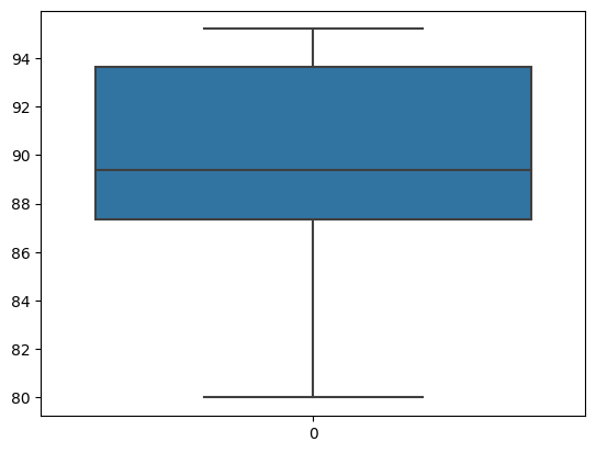
np.mean(A1)73.49111111111111