[25-1 Winter Session 7] Brownian Motion

8.1 Introduction

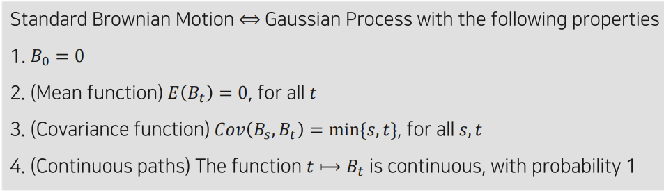
Standard Brownian Motion

📌

Notation

• ($B_t)_{t\geqq 0}$ : 연속시간 Stochastic Process - 표준 Brownian motion

• $B_t$ : 시간 t 에 입자의 무작위 위치 $x$

• $P(B_t\leq z)$ : 시간 t에 움직인 정도가 $z$ 보다 작을 확률

• 1차원 브라운 운동 - 위치는 반드시 $\mathbb{R}$ 실수선 위에서 움직임
• $\mathbb{R}^n$ 고차원으로 확장 가능 → $\mathbf{B}_t = (B_t^{(1)},\dots,B_t^{(n)})$ 각각의 성분이 1차원 표준 브라운 운동,

---

Definition

• 아래 5가지를 만족하면 표준 Brownian motion를 만족

1. $B_0=0$ # 원점 스타트

2. Normal Dist. : $B_t$ , 시점 t의 위치가 평균 0 분산이 t 인 정규분포를 따름

   $B_t\sim\bold{N}(0,t)$

3. Stationary Inc : 시작시간이 0이든, s 든 상관없이 얼마나 움직였는지의 $B$ 차이는 더 흐른 시간 s에만 의존한다. - poisson process 의 stationary와 동일 (z 가 이산 정수인지, 실수인지만 다름)

   $P(B_{t+s} - B_s \leq z) = P(B_t \leq z) = \int_{-\infty}^{z} \frac{1}{\sqrt{2\pi t}} e^{-x^2/2t} \,dx$

4. Independent inc : 겹치지 않는 시간구간 간의 변위는 서로 독립이다 ( 역시 포아송 과정과 동일)

1. Continuous : $t→B_t$ 함수가 연속적이어야 함.
   → 이동과정에서 끊김이 없고, 부드럽게 움직인다는 것을 위치함수의 연속성으로 설명

---

Continuous Markov Chain 과 Poisson, Brownian Motion 의 관계?

• Markov Property : 무기억성 - 조건부 독립

  $P(Xt+h∈A(Xu)u≤t)=P(Xt+h∈AXt).$
  • 조건부 독립 - 현재 상태가 주어졌을 때, 미래값이 정해짐, 즉 겹치지 않는 시간이 아예 무관하다는 것을 보장하지 않음

• Independent increments : 독립증분

  • 겹치지 않으면 무조건 독립

• Independent inc 면 Markov Property를 항상 가지지만, 그 역은 항상 참은 아님

  • Brownian motion이나 Continuous MC는 Ind inc 면서 Markov Property 만족

  • 고객이 1명인 상태의 Markov Chain 대기행렬 (M/M/1) 등은 markov property를 가지지만 독립 증분을 만족하지 않음. (고객 도착시간, 서비스 시간 모두 지수분포, 서버는 1명)

    → 겹치지 않는 시간대라도 대기시간 $W_q$ 는 이전 시간의 고객 수에 연관

---

예제 2. $\displaystyle P\bigl(B_s \le 3 \,\big|\; B_2 = 1\bigr)$

$\displaystyle P(B_3 \le 2)$

독립증분 & 마코프성

• 표준 브라운 운동은 “독립증분”과 “MarkovProperty” 만족
• 시점 t=2에서 $B_2=1$이 주어져 있으면, 그 이후 $(B_s - B_2)$는 조건부로 새로 시작하는 브라운 운동과 같은 분포가 됨

포아송 과정과 동일

예제 3. $\displaystyle \mathrm{Cov}(B_s, B_t)=?$

$\mathrm{Cov}(B_s, B_t) = \min(s,t) = s$

• 증명 : $Cov(B_s,B_t)=E[B_sB_t]−E[B_s]E[B_t]=E[B_sB_t]$
  $(E[B_s]=E[B_t]=0).$
• 그런데 $B_t=B_s+(B_t−B_s)$ 이고, $B_s와 (B_t−B_s)$ 가 독립이므로 $\mathbb{E}[\,B_s B_t\,] = \mathbb{E}[\,B_s \,\bigl(B_s + (B_t - B_s)\bigr)\,] = \mathbb{E}[\,B_s^2\,] + \mathbb{E}[\,B_s\, (B_t - B_s)\,].$
  
• 앞서 def 에서 $B_t$ 는 모든 t에서 평균 0 분산 t 인 정규분포를 따름
• 따라서 $Cov(B_s,B_t) = min(s,t)=s$ 로 겹치는 구간 중 작은 구간의 길이 s

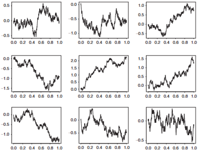
Simulation of Brownian Motion

구간 [0,t] 를 n개의 시점으로 균등분할해, 각 n개의 시점의 위치변수를 생성하고 다음과 같이 정의

→ $B_{t1} , B_{t2} , … , B_{tn}$

독립증분과 정상증분을 이용해 $X_i$ 라는 B와 독립된 R.V 생성

$B_{t_i} = B_{t_{i-1}} + (B_{t_i} - B_{t_{i-1}})\xrightarrow{d} B_{t_{i-1}} + X_{i}$

$X_i \sim N(0,t_i-t_{i-1})$ , 즉 $X_i \sim N(0,\frac{t}{n})$

따라서 $B_{t_i}$ 는 그전 time 단위의 변위 $B_{t_{i-1}}$ 에 표준정규분포 * $\sqrt{\frac{t}{n}}$ 곱한 변수를 계속 더하는 방식

결국 아래와 같이 표기 가능

$B_{t_i} = B_{t_{i-1}} + \sqrt{\frac{t}{n}}Z_i, \quad \text{for } i = 1, 2, \ldots, n$

결국 시뮬레이션은 잘게 쪼갠 $\frac{t}{n}$ 의 시간 step 마다 $\frac{t}{n}$ 에 비례한 크기로 정규분포를 따르는 변위 변화량을 샘플링함.

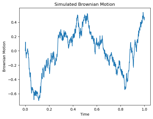
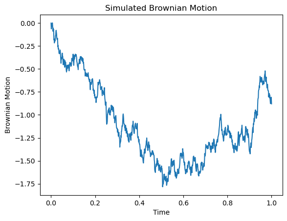
시뮬레이션

import numpy as np
import matplotlib.pyplot as plt

# 파라미터 설정
n = 1000  # 스텝 수
t = 1     # 전체 시간
dt = t / n

# 브라운 운동 시뮬레이션: 첫 값 0에 이어서 정규분포 난수의 누적합
increments = np.random.normal(0, np.sqrt(dt), n)
bm = np.concatenate(([0], np.cumsum(increments)))

# 시간 스텝 생성
steps = np.linspace(0, t, n + 1)

# 결과 플롯
plt.plot(steps, bm)
plt.xlabel("Time")
plt.ylabel("Brownian Motion")
plt.title("Simulated Brownian Motion")
plt.show()

그냥 짧은 시간단위로 시간 길이에 비례하는 정규분포 R.V 값 계속 더하면 시뮬레이션이 되네?

→ 그렇게 Random Walk 와 Gausian Process 연결

8.2 Brownian Motion

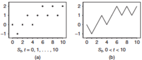
< Random Walk >

이산적 step 마다 1/2 확률로 1 or -1 을 더하는 sequence

시작 값 0, 최종 값은 각 step의 더하는 값 R.V : $X_i$ 의 합에 의해 결정됨

${S_t}$: Discrete-time Discrete-state Random Walk

• $X_1, X_2, ...$ 는 각각 1/2 의 확률로 ±1 의 값을 가지는 iid sequence
• $S_0 = 0$
• $S_t = X_1 + ... + X_t$

< Brownian Motion간의 유사성 >

• $S_0 = 0$
• $S_t ≈ N(0,t)$ by CLT $( E(S_t) = 0, Var(S_t) = t )$
• $S_{t+s} - S_s = X_{s+1} + ... + X_{t+s} d= S_t$
• $S_t - S_s$ and $S_r - S_q$ are independent
• 함수연속성만 다름

$E(S_t)=0, Var(S_t)\approx t$ → Brownian motion 과 비슷하다~

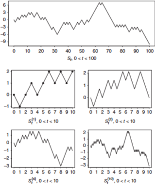
원래 random walk 보다 스케일링 시켜, 같은 시간동안 n배 많은 walk 이 있다고 하자,

결국 Random Walk 라는 discrete state process 는 $n→ \infin$ 일 때 Brownian Motion으로 수렴한다.

증명 생략

$S_t^{(n)}$ : 시점 t에서의 값 $S_t$ 가 n배 스케일링 됨.

n 이 커질수록 brownian 형태를 띔

8.3 Gaussian Process

1. 브라운 운동이 가우시안 과정이 됨을 확인
2. 가우시안 과정이 브라운 운동이 되기 위한 조건 확인

이런 선형조합이 정규분포를 따르면, 확률변수열 $X_1…X_k$ 는 다변량 정규분포를 가짐.

def : Gausian Process

• 평균, 분산, pdf

$\mu = (\mu_1, \ldots, \mu_k) = (E(X_1), \ldots, E(X_k))$

$V_{ij} = \text{Cov}(X_i, X_j), \quad \text{for } 1 \leq i, j \leq k.$

$f(x) = \frac{1}{(2\pi)^{k/2} |V|^{1/2}} \exp\left(-\frac{1}{2}(x - \mu)^T V^{-1} (x - \mu)\right)$

A Gaussian process $(X_t)_{t≥0}$ 는 모든 $n=1,2…$ 에 대해 $0 ≤ t_1 < · · · < t_n$ 를 만족하는 경우 R.V $X_{t1}… X_{tn}$ 이 다변량 정규분포를 따르는 Continuous time stochastic process 임.

Gaussian Process 는

• mean function $E(X_t), for\ t ≥ 0$,
• covariance function $Cov(X_s, X_t)$, $for \ s, t ≥ 0$

이 둘에 의해 완전히 결정됨.

가우시안 → 브라운 조건

1. $B_0=0$
2. mean function은 모든 t에서 0
3. Cov function은 모든 s,t 에서 min(s,t)
4. 함수 연속성

→ 그냥 2번 정규성 조건만 가우시안 과정이라 맞췄으니까 1,3,4,5 조건 맞추면 Brownian motion 이란 말.

• Nowhere Differentiable paths : 브라운 운동의 경로는 전 구간 미분 불가

8.4 Transformations and Properties

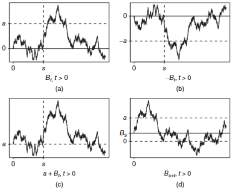
브라운 운동의 변환. 표준 브라운운동을 변환해도 그대로 브라운 운동

Let $(B_t)_{t≥0}$ be a standard Brownian motion. Then, each of the following transformations is a standard Brownian motion.

• Reflections 대칭이동

  • (Relection) $(−B_t)_{t≥0}.$

• Translation 평행이동 - 시간 s 만큼 이동 -

  • $(B_{t+s} − B_s)_{t≥0}$
  • 무기억성, stationary

• Rescaling - 스케일링 -

  • $(a^{-1∕2}B_{at})_{t≥0}, \text{for all }a > 0.$

• Inversion -

  • The process $(X_t)_{t≥0}$ deined by $X_0 = 0$ and $X_t = tB_{1∕t}$, for t > 0.

• 변환 예시

Property :

1. Markov Property

• discrete-time discrete-state : $P(X_{n+1} = j | X_0 = x_0, ..., X_{n-1} = x_{n-1}, X_n = i) = P(X_{n+1} = j | X_n = i)$
• continuous-time discrete-state : $P(X_{t+s} = j | X_s = i, X_u = x_u, 0 \leq u \leq s) = P(X_{t+s} = j | X_s = i)$
• continuous-time continuous-state : $P(X_{t+s} \leq y | X_u, 0 \leq u \leq s) = P(X_{t+s} \leq y | X_s)$ → Brownian Motion은 만족

1. Transition Matrix/Function/Kernel (when time homogeneous)

• discrete-time discrete-state : $P_{ij} = P(X_1 = j | X_0 = i)$ (현재 상태일 때 다음 상태가 j일 확률)
• Continuous-time discrete-state : $P_{ij}(t) = P(X_t = j | X_0 = i)$ (현재 상태일 때 t시간 후 j상태일 확률)
• Continuous-time continuous-state : $K_t(x,y) = \frac{1}{\sqrt{2\pi t}} e^{-(y-x)^2 / 2t}$ (초기 위치가 x일 때 t시간 후 X_t의 위치 y의 분포) (Brownian Motion)

1. Distribution

• discrete-time discrete-state : $\alpha P^n$ (초기분포 \alpha, n시점 후의 분포)
• Continuous-time discrete-state : $\alpha P(n)$ (초기분포 \alpha, n시간 후의 분포)
• Continuous-time continuous-state : $K_n(x,y) = \frac{1}{\sqrt{2\pi n}} e^{-(y-x)^2 / 2n}$ (초기 위치가 x, n시간 후의 분포)

(Brownian motion)

• discrete-state의 경우에는 특정 시점/시간 후에 특정 상태에 있을 확률들이 제시됨
• continuous-state의 경우에는 특정 시간 후에 특정 위치에 있을 확률 대신, 특정 시간 후의 위치의 분포가 제시됨
  • $P(X_t \leq y | X_0 = x_0) = \int_{-\infty}^{y} K_t(x_0, w) dw$
• Markov property를 활용하여 다양한 확률계에 대한 통계적 분석이 가능함
  • $T_a = \min \{t: B_t = a\}$의 분포 $/ M_t = \max_{0 \leq s \leq t} B_s$의 분포
  • z_{T,t} = P(at least one zero in (T,t))의 값 / L_t = last zero in (0,t)의 분포

n스텝 후 $\alpha P^n$ 이 분포 →

αPn로 분포 기술

Continuous time Discrete state

생성행렬

브라운 운동 :

$K_t(x,y) = \frac{1}{\sqrt{2\pi t}} e^{-\frac{(y-x)^2}{2t}}$

---

8.5. Variations and Applications

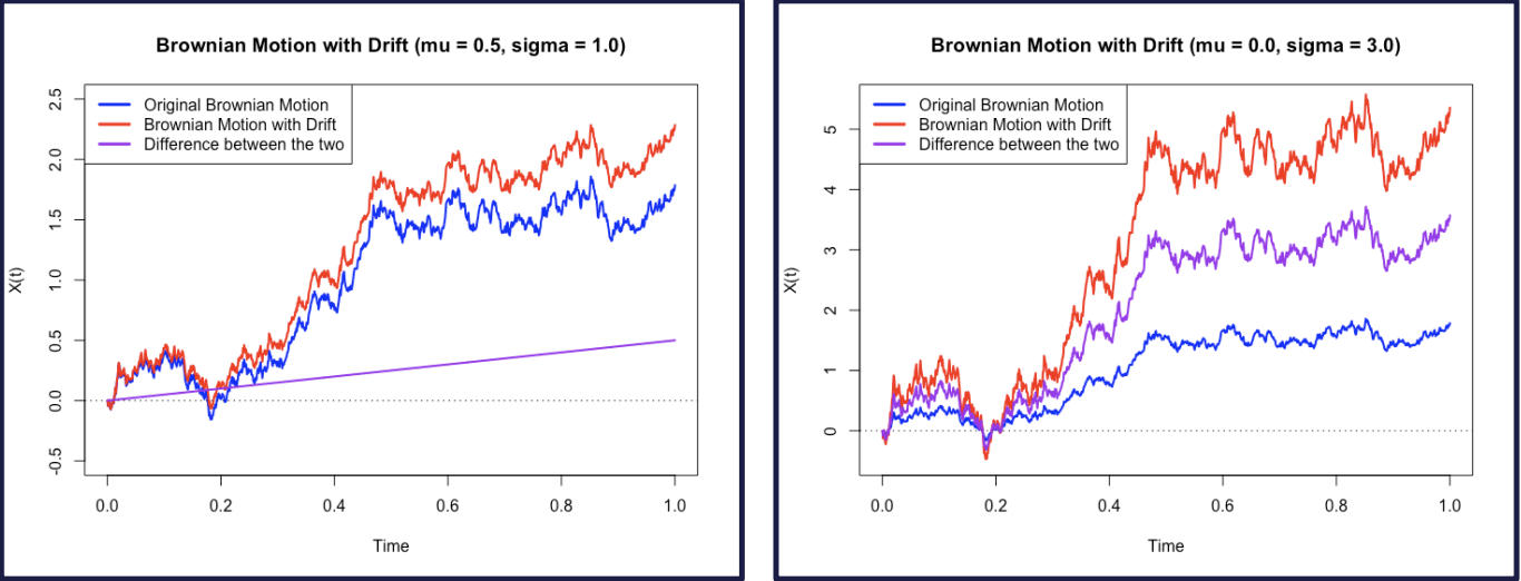
Brownian Motion with Drift

For real $\mu$ and $\sigma >0$, the process defined by

$X_t= \mu t+ \sigma B_t$ , for $t\geq0$

drift parameter: $\mu$

variance parameter: $\sigma^2$

example 8.11

Q: 스포츠 게임에서의 Home Team이 게임에 대한 이득이 있을까?

$l:$ Home team point advantage

$t:$ Time of match, $0\leq t \leq 1$

$\mu:$ Measure of Home Team advantage

$X_t :$ Difference in scores after 100t percent of the game has been completed

$p(l,t)=P(X_1>0|X_t=l)=P(X_1-X_t>-l)$

         $=P(X_{1-t}>-l)=P(\mu(1-t)+\sigma B_{1-t}>-l)$

         $=P(B_{1-t}<\frac{l+\mu(1-t)}{\sigma})$

         $=P(B_t<\frac{\sqrt{t}[l+\mu(1-t)]}{\sigma\sqrt{1-t}})$    $\leftarrow$여기 넘어가는거는 모르겠어요!!

Brownian Bridge

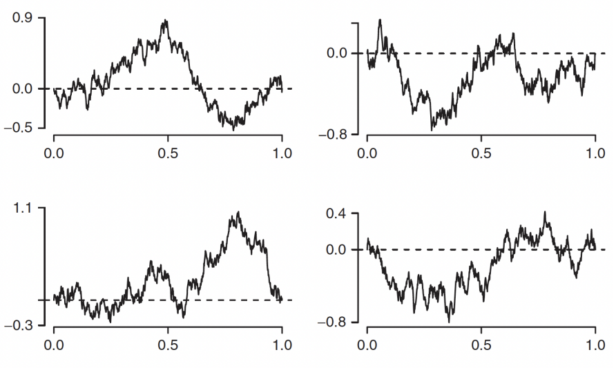
From standard Brownian Motion, the conditional process $(B_t)_{0\leq t \leq1}$ given that $B_1=0$

example 8.12

Let $X_t=B_t-tB_1,$ for $0\leq t\leq1$. Show that $(X_t)_{0\leq t\leq1}$ is a Brownian bridge

Solution

SInce $X_t$ is a linear transformation of Gaussian Process $(B_t)_{t\geq0}$, it is also a Gaussian Process

1. $X_0=B_0=0$

2. $E[X_t]=E[B_t-tB_1]=E[B_t]-tE[B_1]=0$

3. $Cov(X_s,X_t)=E(X_sX_t)=E((B_s-sB_1)(B_t-tB_1))$

                        $=E(B_sB_t)-tE(B_sB_1)-sE(B_tB_1)+stE(B_1^2)$
   
                         $=min(s,t)-ts-st+st=min(s,t)-st$

Geometric Brownian Motion

Let $(X_t)_{t\geq0}$ be a Brownian Motion with draft parameter $\mu$ and variance parameter $\sigma^2$

The process $(G_t)_{t\geq0}$ defined by

$G_t=G_0e^{X_t}$, for $t\geq0$

where $G_0>0$ , is called Geometric Brownian Motion

More Formal Definition

$dG_t=\mu G_tdt+\sigma G_tdW_t$

distribution?

$\ln{G_t}=\ln{G_0}+X_t$

$E[\ln{G_t}]=E[\ln{G_0}+X_t]=\ln{G_0}+\mu t$

$Var(\ln{G_t})=Var(\ln{G_0}+X_t)=Var(X_t)=\sigma^2t$

for each $t>0$, $G_t$ has a log-normal distribution

example 8.15

stock price가 Geometric Brownian Motion으로 model되는 이유

• 장기적으로 Exponential Growth/Decline이 대부분의 주식
• 가격은 음수일 수 없으며, Geometric Brownian Motion은 양수만 받는다
• 특정 날의 가격과 다음날의 가격은 독립이 아닐 수 있지만 Day to Day Percent Changes는 iid하게 모델링 가능

8.6 Martingales

우리가 게임을 하고 있을 때 얻는 이득이 stochastic process라고 하면, 이게 fair game 이라는 notion을 generalize하는게 martingale

fair game= expected future winnings가 past history와 무관

discrete-time martingale $Y_0,Y_1,\cdots$에서는

1. $E[Y_{n+1}|Y_0,\cdots,Y_n]=Y_n$
2. $E[|Y_n|]<\infty$

important property

$E[Y_t]=E[E[Y_t|Y_r,0\leq r\leq s]]=E[Y_s],0\leq s\leq t$

$E[Y_t]=E[Y_0],\forall t \in[T]$

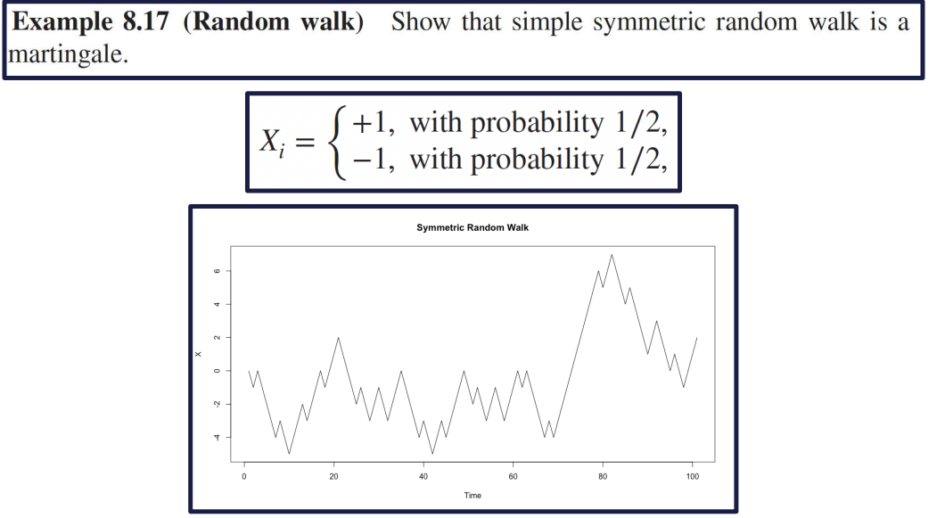
example 8.17 (Random Walk)

Let $S_n=X_1+\cdots+X_n$, $S_0=0$

$E(S_{n+1}|S_0,\cdots,S_n)=E(X_{n+1}+S_n|S_0,\cdots,S_n)$

                                        $=E(X_{n+1}|S_0,\cdots,S_n)+E(S_n|S_0,\cdots,S_n)$

                                        $=E(X_{n+1})+S_n=S_n$

using Jensen’s inequality

$E(|S_n|)=E(|\Sigma^n_{i=1}X_i|)\leq E(\Sigma^n_{i=1}|X_i|)=n<\infty$

Martingale with Respect to Another Process

Let $(X_t)_{t\geq0}$ and $(Y_t)_{t\geq0}$ be stochastic process. Then $(Y_t)_{t\geq0}$ is a martingale with respect to $(X_t)_{t\geq0}$, if for all $t\geq0$

$Y_t=g(X_t)$이라고 하면 많이 사용됨

$X_t$를 s까지의 과거의 정보라고 생각

example 8.19

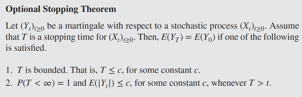
Optional Stopping Theorem

First Hitting time: a단계에 처음 도달하는 시간

Martingale은 모든 Fixed time에 대해서의 기댓값이 같아야한다. Random time에서는 해당되지 않음

example (Gambler’s Ruin)

1 franc을 이기면 얻고 지면 잃는 게임

베팅 전략: 이기면 멈추고 지면 판돈을 두배로

T: 이길 때까지의 판수(a.k.a Stopping time)

k번만큼 했으면

$2^k-(1+2+\cdots+2^{k-1})=2^k-(2^k-1)=1$

확률 1로 이기기에 T가 Winning Stragedy로 보이지만

$E[Y_t]=1\neq0=E[Y_0]$이므로 Optional Stopping Theorem에 만족하지 않음

무한 자산이 아니기에 Winning Stragedy가 아님

example 8.22

$T=min(t:B_t=a ~~or~~B_t=-b)$