이번 시간에는 기존의 머신러닝과 다르게 '스스로 학습할 수 있도록 만드는 신경망'인 딥러닝을 학습했고, 이를 이해하기 위해 OR게이트와 XOR게이트를 구현해봤다.
1.OR게이트 구현하기
1-1) 문제정의
- OR 게이트 구현 [0,0] -> 0, [1,0] -> 1, [0,1] -> 1, [1,1] -> 1
- 즉, 둘 다 0이면 0 출력, 하나면 0이면 1 출력, 둘 다 1이면 1을 출력한다.
1-2) 데이터 준비하기
#라이브러리 임포트
import tensorflow as tf
tf.random.set_seed(777) # 똑같은 데이터 셋을 활용할 수 있도록 고정

import numpy as np
from tensorflow.keras.models import Sequential
from tensorflow.keras.layers import Dense
from tensorflow.keras.optimizers import SGD
from tensorflow.keras.losses import mse

#데이터 준비하기
data = np.array([[0,0], [1,0], [0,1], [1,1]])
label = np.array([[0],[1],[1],[1]])- data는 문제지인 X값, label는 답안지인 y값이다.
1-3) 모델 구성하기
model = Sequential()
model.add(Dense(1, input_shape=(2,), activation='linear')) # -> 단층 퍼셉트론- 하나의 레이어 당 신경망의 갯수를 몇 개 사용할지 Dense에 넣어주자
- 한개를 쓴다는 건 결정경계를 하나만 쓰겠다는 것
- input_shape은 input_shap=(2,)의 형태로 input_dim은 input_dim=2의 형태로 작성한다.
#activiation: 활성화 함수 linear로 설정
1-4) 모델 설정하기
model.compile(optimizer=SGD(), loss=mse, metrics=['acc'])- 가중치 값을 변경하도록 결정하는 옵티마이저이자 역전파 알고리즘은 SGD로 사용
- mse(mean square error): 차이를 제곱 후 더해서 평균낸 값; 즉, 오차의 정도를 알려줌
- 정확도를 학습할 때마다 acc로 메트릭스에 넣어줘
1-5) 모델 학습하기
history = model.fit(data, label, epochs=500) - data는 X값, label은 Y값이며, epochs는 해당 모델을 몇 번 학습할지 정하는 값이다.
- 이 epochs별로 손실값(오차)과 정확도를 알아볼 수 있으며, 손실값이 점차 상승하거나 정확도가 떨어진다면 조절이 필요하다는 것을 알 수 있다.
- history는 학습한 결과를 변수에 담아 차후 학습횟수별 오차와 정확도를 차트로 그리는 등 활용할 수 있게 저장해 놓는 것이다.
1-6) 학습결과 그려보기
import matplotlib.pyplot as plt

his_dict = history.history
loss = his_dict['loss']

epochs = range(1, len(loss) + 1)
fig = plt.figure(figsize = (10, 5))

# 훈련 및 검증 손실 그리기
ax1 = fig.add_subplot(1, 2, 1)
# 가로 한줄 세로 두줄로 그릴 건데 얘는 첫번째 차트야
ax1.plot(epochs, loss, color = 'orange', label = 'train_loss')
ax1.set_title('train loss')
ax1.set_xlabel('epochs')
ax1.set_ylabel('loss')
ax1.legend()

acc = his_dict['acc']

# 훈련 및 검증 정확도 그리기
ax2 = fig.add_subplot(1, 2, 2)
# 가로 한줄 세로 두줄로 그릴 건데 얘는 두번째 차트야
ax2.plot(epochs, acc, color = 'blue', label = 'train_accuracy')
ax2.set_title('train accuracy')
ax2.set_xlabel('epochs')
ax2.set_ylabel('accuracy')
ax2.legend()

plt.show()- 이해하는대로 주석을 추가할 예정
2.XOR게이트 구현하기
2-1) XOR게이트 단층 퍼셉트론으로 구현 -> 실패
#데이터 준비하기

data = np.array([[0,0], [1,0], [0,1], [1,1]])
label = np.array([[0],[1],[1],[0]])

#모델 구성, 설정 및 학습하기
xor0_model = Sequential()
xor0_model.add(Dense(1, input_shape=(2,), activation='linear'))
xor0_model.compile(optimizer=SGD(), loss=mse, metrics=['acc'])

history = xor0_model.fit(data, label, epochs=500) - XOR게이트에서는 두 값이 같을 경우 0을, 두 값이 다르면 1을 출력한다.
- 선형함수를 쓰는 건 층을 쌓는 의미가 없어져버림 즉, f(f(f(x))) -> f(x)
import matplotlib.pyplot as plt

his_dict = history.history
loss = his_dict['loss']

epochs = range(1, len(loss) + 1)
fig = plt.figure(figsize = (10, 5))

# 훈련 및 검증 손실 그리기
ax1 = fig.add_subplot(1, 2, 1)
ax1.plot(epochs, loss, color = 'orange', label = 'train_loss')
ax1.set_title('train loss')
ax1.set_xlabel('epochs')
ax1.set_ylabel('loss')
ax1.legend()

acc = his_dict['acc']

# 훈련 및 검증 정확도 그리기
ax2 = fig.add_subplot(1, 2, 2)
ax2.plot(epochs, acc, color = 'blue', label = 'train_accuracy')
ax2.set_title('train accuracy')
ax2.set_xlabel('epochs')
ax2.set_ylabel('accuracy')
ax2.legend()

plt.show()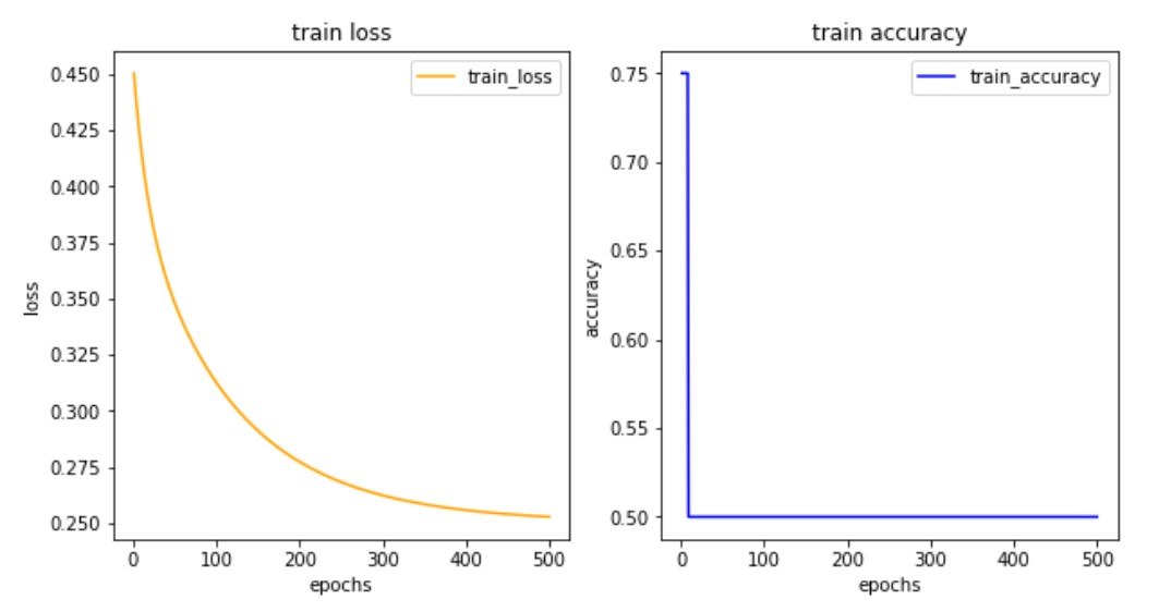
- 정확도 차트를 보면 학습 1회차부터 정확도가 급하락하여 50인 것을 확인할 수 있다.
- 정확도가 50점 이하인 경우 -> 모델이 잘못된 것이며 실패로 간주한다.
- 결론: XOR게이트를 구현하는데 단층 퍼셉트론은 적합하지 않다.
2-2) 다층 퍼셉트론으로 설정 및 활성화 함수/역전파 알고리즘 변경
#데이터 준비하기
data = np.array([[0,0], [1,0], [0,1], [1,1]])
label = np.array([[0],[1],[1],[0]])

from tensorflow.keras.optimizers import RMSprop

xor_model = Sequential()
xor_model.add(Dense(32, input_shape=(2,), activation='relu')) # input층이면서 첫번째 레이어
xor_model.add(Dense(1, activation='sigmoid'))
# 첫번째 층에서 입력받아서 출력해주는 두번째 레이어 결과를 한개만 낼 것이라서 1 입력
xor_model.compile(optimizer=RMSprop(), loss=mse, metrics=['acc'])
# 손실점수는 mean square error를 사용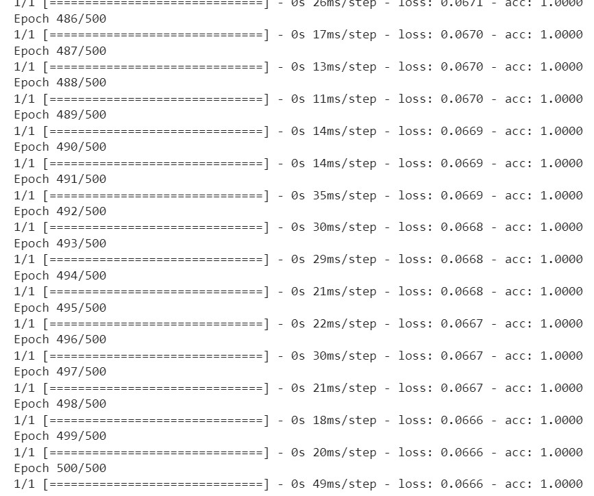
history = xor_model.fit(data, label, epochs=100)- 단층 퍼셉트론 대신 다층 퍼셉트론을 사용하자
- 하나의 레이어 당 신경망의 갯수를 32개 사용한다는 것 -> 'Dense(32,'
- 다층 퍼셉트론은 레이어를 여러 개 사용하며 첫번째 층에서 내린 결과를 두번째 층에 가중치를 부여해 결과 값을 전달한 후 마지막 층에서 출력해 정확한 예측이 가능
- 신경망의 갯수는 2의 제곱의 형태로 사용하는 것이 성능이 좋다고 논문에서 밝혀짐 일반적으로 데이터가 방대할수록 숫자를 크게 줌
- 첫 add층(레이어) = 입력층
- 마지막 add층(레이어) = 출력층
- 히든 레이어 = 내부적으로 일하는 층
- input_shape: 내가 가진 feature의 개수
- mse = (예측값-정답)의 제곱값 = 오차율이 점점 줄게 하는 것이 목표
- 이 손실 점수(mse)를 optimizer에게 주고 이 옵티마이저가 각 레이어에서 가중치를 조정한다.
- 활성화함수: 각 퍼셉트론마다 하나의 활성화 함수를 사용하는데 가중치들을 sum하고 다음 레이어로 y값을 보낼 때 어떤 값으로 보낼지 결정하는 함수를 말한다.
- input이나 중간 층들은 'relu'를 사용한다. -> 구간을 tight하게 줌 (즉, 의견을 강력하게 어필하는 스타일)
- 결과 층들은 'sigmoid'를 사용한다. -> 구간을 rough하게 줌 그 이유, 우리의 목표는 일반화된 모델을 만들어야 하기 때문
- 하이퍼볼릭 탄젠트(tanh)는 sigmoid와 relu의 중간 정도의 활성화 함수
- 결국 내가 데이터를 명확하게 알고 문제정의를 정확하게 해야 모델을 커스터마이징 할 수 있다.
#학습결과 차트 그리기
import matplotlib.pyplot as plt

his_dict = history.history
loss = his_dict['loss']

epochs = range(1, len(loss) + 1)
fig = plt.figure(figsize = (10, 5))

# 훈련 및 검증 손실 그리기
ax1 = fig.add_subplot(1, 2, 1)
ax1.plot(epochs, loss, color = 'orange', label = 'train_loss')
ax1.set_title('train loss')
ax1.set_xlabel('epochs')
ax1.set_ylabel('loss')
ax1.legend()

acc = his_dict['acc']

# 훈련 및 검증 정확도 그리기
ax2 = fig.add_subplot(1, 2, 2)
ax2.plot(epochs, acc, color = 'blue', label = 'train_accuracy')
ax2.set_title('train accuracy')
ax2.set_xlabel('epochs')
ax2.set_ylabel('accuracy')
ax2.legend()

plt.show()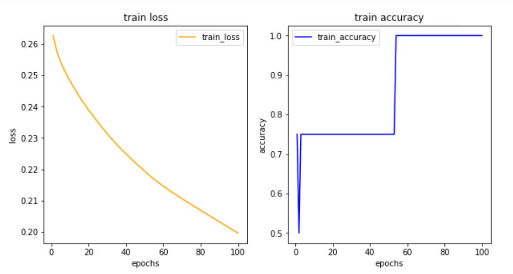
- 학습결과나 차트를 확인했을 때, 손실값이 가파르게 떨어지면 더 떨어질수도 있기 때문에 정확도를 높일 수 있는 상태이므로 학습 횟수를 늘려준다.