다층 퍼셉트론 이진 분류
1. 피마족 인디언 당뇨병 발병 유무 예측
1) 문제정의
- 피마족 인디언 당뇨병 발병 유무를 예측하는 이진 분류 문제(당뇨병:1 , 정상:0)
2) 데이터 준비하기
#라이브러리 임포트
import numpy as np
import pandas as pd
from sklearn.model_selection import train_test_split

import tensorflow as tf
from keras.models import Sequential
from keras.layers import Dense

#랜덤씨드 고정
np.random.seed(5)

dataset = pd.read_csv('/content/drive/MyDrive/Colab Notebooks/diabetes.csv')
3) 데이터 분리하기
X= dataset[['Pregnancies', 'Glucose', 'BloodPressure', 'SkinThickness', 'Insulin',
       'BMI', 'DiabetesPedigreeFunction', 'Age']]
y = dataset['Outcome']

# 정규화
from sklearn import preprocessing
X = preprocessing.StandardScaler().fit(X).transform(X)

# 훈련과 테스트 비율 8:2
X_train, X_test, y_train, y_test = train_test_split(X, y, test_size=0.2,
                                                    random_state = 777)
4) 모델 구성하기
model = Sequential()
model.add(Dense(32, input_dim=8, activation = 'relu'))
model.add(Dense(8, activation = 'relu'))
model.add(Dense(1, activation = 'sigmoid'))
#모델의 구성 확인하기
model.summary()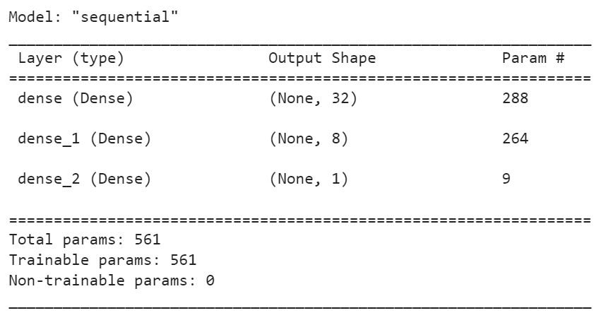
#모델의 구성을 그림으로 확인
tf.keras.utils.plot_model(model, show_shapes=True, show_layer_names=True,
                          rankdir='TB', expand_nested=False, dpi =100)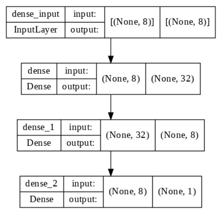
5) 모델 설정하기
model.compile(loss='binary_crossentropy', optimizer='adam', metrics=['acc'])6) 모델 학습하기
history = model.fit(X_train, y_train, epochs=1500, batch_size=128)- 'batch_size = 128'의 의미는 모든 학습회차 동안 128개의 데이터를 단위로 가중치를 반환해달라는 뜻이다. 학습 1회차 씩 수행하고 가중치를 반환해 넘어가면 반영해야 할 가중치 변화를 놓칠 수 있기 때문.
- 만약 데이터 수가 256개라면, 128개 학습하고 가중치 변경, 나머지 128개하고 가중치 변경하라는 의미
7) 모델 평가하기
scores = model.evaluate(X_train, y_train)
# 손실점수 값과 정확도 두개 값을 주기에 scores
print(model.metrics_names[0], scores[0])
print('%s: %.2f%%' % (model.metrics_names[1], scores[1]*100))- 결과값: 20/20 - 0s 2ms/step - loss: 0.3740 - acc: 0.8404
loss 0.3740347921848297
acc: 84.04%
8) 학습결과 그리기
#학습결과 그려보기

import matplotlib.pyplot as plt

his_dict = history.history
loss = his_dict['loss']

epochs = range(1, len(loss) + 1)
fig = plt.figure(figsize = (10, 5))

# 훈련 및 검증 손실 그리기
ax1 = fig.add_subplot(1, 2, 1)
ax1.plot(epochs, loss, color = 'orange', label = 'train_loss')
ax1.set_title('train loss')
ax1.set_xlabel('epochs')
ax1.set_ylabel('loss')
ax1.legend()

acc = his_dict['acc']

# 훈련 및 검증 정확도 그리기
ax2 = fig.add_subplot(1, 2, 2)
ax2.plot(epochs, acc, color = 'blue', label = 'train_accuracy')
ax2.set_title('train accuracy')
ax2.set_xlabel('epochs')
ax2.set_ylabel('accuracy')
ax2.legend()

plt.show()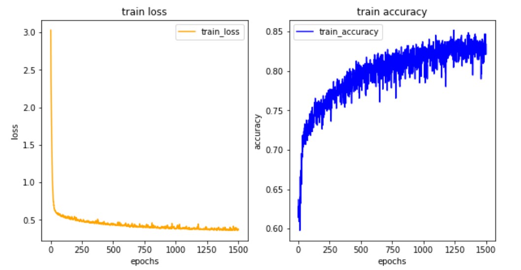
- 손실값은 떨어지고 정확도는 높아짐 -> 공부를 잘 하고 있구나^0^라고 판단 가능
2. 폐암 수술 환자의 생존 유무 예측하기
1) 문제정의
- 폐암 수술 환자의 생존 유무를 예측하는 이진 분류 문제로 정의(생존:1, 사망:0)
2) 데이터 준비하기
#라이브러리 임포트
import numpy as np
import pandas as pd
from sklearn.model_selection import train_test_split

import tensorflow as tf
from keras.models import Sequential
from keras.layers import Dense

#랜덤씨드 고정
np.random.seed(5)

#데이터 읽어오기
dataset = pd.read_csv('/content/ThoraricSurgery.csv', header=None)- 원시자료를 보고 컬럼명이 없다는 것을 확인했기 때문에 None으로 작성
3) 데이터셋 분리하기
- 입력값(feature = 17개), 출력값(label = 1개)
X = dataset.iloc[:,:-1] #마지막 열이 결과 값이니까 그 열 제외하고 데려와
y = dataset.iloc[:,-1]- X값: 행은 전체, 열은 전체 중 1개 열만 빼고 담기
- y값: 행은 전체, 열은 맨 뒤 열만 담기
X_train, X_test, y_train, y_test = train_test_split(X, y, test_size=0.1,
                                                    random_state=7)
4) 모델 구성, 설정 및 학습하기
model = Sequential()
model.add(Dense(30, input_dim=17, activation = 'relu'))
model.add(Dense(20, activation='relu'))
model.add(Dense(10, activation='relu'))
model.add(Dense(1, activation='sigmoid'))

model.compile(loss='binary_crossentropy', optimizer='adam', metrics=['acc'])

history = model.fit(X_train, y_train, epochs=100, batch_size=64) - 64씩 결과보다가 가중치 변경해줘 423(Xtrain 개수/64 = 6.XXXXX 423 건 중에 64건 먼저 하고 또 64건 하고 그 다음 64건 공부해
- 데이터 셋 크기가 작을 때는 배치 사이즈를 정해주지 않아도 됨 -> 즉, 한 번에 학습해서 가중치 변경이 잘 될 때는 정해주지 않아도 됨
- 배치 사이즈를 설정한다는 건 세세하게 중간중간 정리할 시간을 주면서 가중치를 업데이트 시킬 수 있도록 하는 것
- 따라서 데이터 크기가 큰 경우 배치 사이즈를 주는 것이 좋음
#학습결과 그려보기
import matplotlib.pyplot as plt

his_dict = history.history
loss = his_dict['loss']

epochs = range(1, len(loss) + 1)
fig = plt.figure(figsize = (10, 5))

# 훈련 및 검증 손실 그리기
ax1 = fig.add_subplot(1, 2, 1)
ax1.plot(epochs, loss, color = 'orange', label = 'train_loss')
ax1.set_title('train loss')
ax1.set_xlabel('epochs')
ax1.set_ylabel('loss')
ax1.legend()

acc = his_dict['acc']

# 훈련 및 검증 정확도 그리기
ax2 = fig.add_subplot(1, 2, 2)
ax2.plot(epochs, acc, color = 'blue', label = 'train_accuracy')
ax2.set_title('train accuracy')
ax2.set_xlabel('epochs')
ax2.set_ylabel('accuracy')
ax2.legend()

plt.show()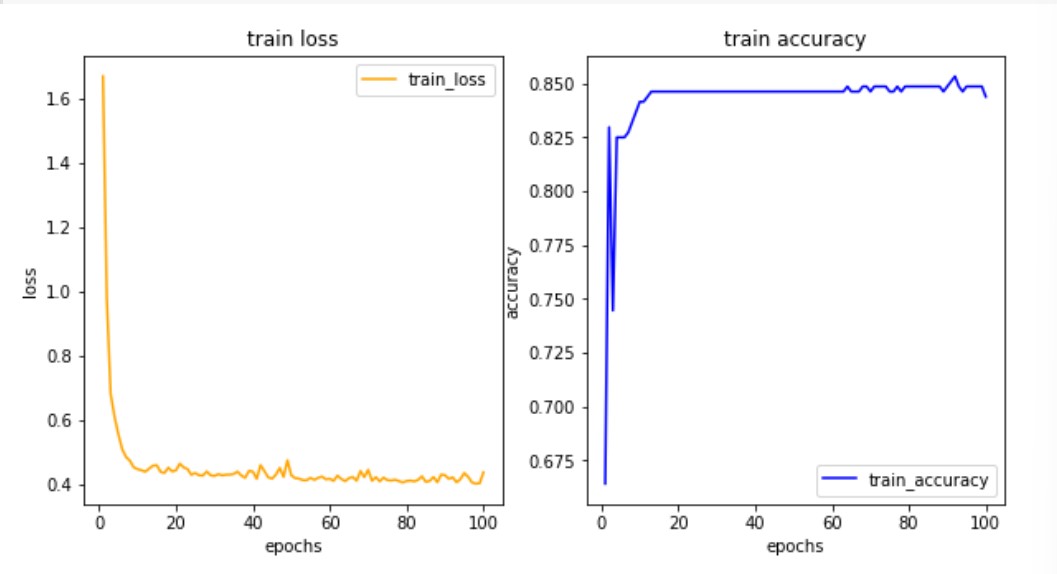
5) 모델 평가하기
scores = model.evaluate(X_train, y_train)
print(model.metrics_names[0], scores[0])
print('%s: %.2f%%' % (model.metrics_names[1], scores[1]*100))

scores = model.evaluate(X_test, y_test)
print(model.metrics_names[0], scores[0])
print('%s: %.2f%%' % (model.metrics_names[1], scores[1]*100))-
결과값
14/14 - 0s 2ms/step - loss: 0.4553 - acc: 0.8487 loss 0.45534735918045044 acc: 84.87% 2/2 - 0s 13ms/step - loss: 0.2934 - acc: 0.8936 loss 0.2933797538280487 acc: 89.36% -
테스트 정확도가 더 높은 이유: 테스트 데이터 수가 작기 때문이라고 추정 가능