소개
- 이 글은 단지 CS231n를 공부하고 정리하기 위한 글입니다.
- Machine Learning과 Deep Learning에 대한 지식이 없는 초보입니다.
- 내용에 오류가 있는 부분이 있다면 조언 및 지적 언제든 환영입니다!
참조
-
https://strutive07.github.io/2019/03/25/cs231n-Lecture-8-1-Deep-Learning-Software.html
-
https://strutive07.github.io/2019/03/25/cs231n-Lecture-8-3-Deep-Learning-Software.html
개요
< Deep Learning Software >
CPU vs GPU
Deep-learning 에서 CPU와 GPU중에 GPU가 더 좋은 이유는 다음과 같습니다.
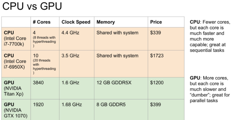
아래 그림을 보시면 CPU는 높은 clock 속도를 가지지만 GPU는 CPU와 비교할 수 없는 Core 수를 가지고 있는 것을 볼 수 있습니다.
결국 GPU가 CPU보다 병렬 계산 처리에 있어서 굉장히 뛰어난 성능을 가지고 있습니다.
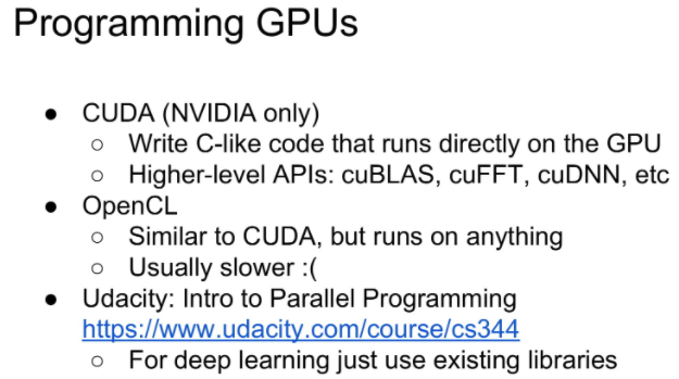
이러한 GPU를 다루기 위해서 사용되는 언어로 유명한 것은 아래와 같습니다.
하지만 머신러닝을 하면서 실제로는 이를 코딩할 일은 거의 없으니 걱정 안하셔도 됩니다.
- CUDA
- OpenCL
- Udacity
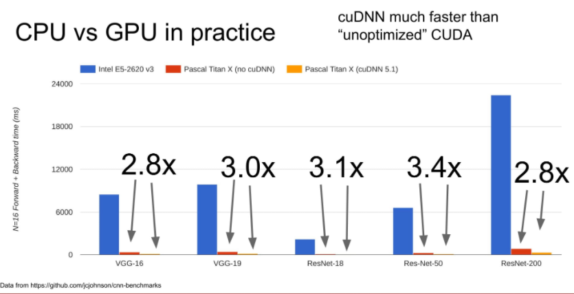
아래 그림을 보면 파란색은 CPU, 빨간색은 GPU, 노란색은 최적화한 GPU를 보여줍니다.
CPU와 그냥 GPU를 비교하면 거의 60~70배 정도가 차이가 난다고 생각하시면 되고,
CUDA를 이용하여 최적화 하면 보통 약 3배정도의 성능 차이를 얻을 수 있다고 합니다.
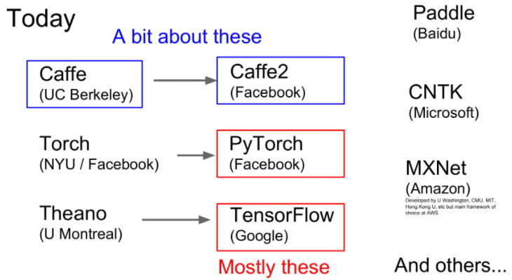
Deep Learning Frameworks
일반적인 유명한 Deep Learning Frameworks로는 Caffe, PyTorch, TensorFlow가 있습니다.
실제 현장과 회사 같은 현업에선느 TensorFlow을 많이 사용하며 연구와 같은 경우 PyTorch를 사용하는 추세라고 합니다.
저는 사실 Pytorch를 사용할 예정이기 때문에 PyTorch에 관련된 내용을 다루겠습니다.
PyTorch
PyTorch에는 3가지 추상화(Abstraction)가 있습니다.
- Tensor : ndarray로, gpu에서 돌아갑니다.
- Variable : computational graph 안에 있는 node 입니다. data와 gradient를 가집니다.
- Module : layer입니다. learnable weight들을 가지거나 state를 저장합니다.
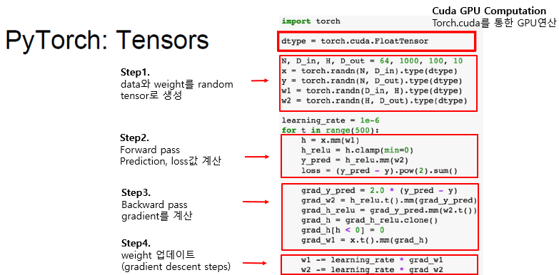
Tensors
아래는 PyTorch에서 사용하는 Tensor 사용법 예시입니다.
Tensor는 GPU에서 사용하는 array입니다.
numpy array와 비슷하지만 GPU에서 돌아간다는 점이 다릅니다.
먼저 dtype이라는 float type의 tensor를 정의하고 이를 type에 넣어주기만 하면 됩니다.
이는 gpu에서 사용할 float array를 만드는 것과 같습니다.
import torch

dtype = torch.cuda.FloatTensor

N, D_in, H, D_out = 64, 1000, 100, 10
x = torch.randn(N, D_in).type(dtype)
y = torch.randn(N, D_out).type(dtype)
w1 = torch.randn(D_in, H).type(dtype)
w2 = torch.randn(H, D_out).type(dtype)
Tensors Autograd
Variable은 node 내부의 data를 말합니다. 대표적으로 weight와 bias가 있습니다.
Variable은 data와 grad를 가집니다. 둘의 shape는 아래와 같습니다.
x.grad.data는 tensor의 gradient 값 입니다.
우리는 입력값 (x, y)에 대해서는 gradient(of loss)가 필요없기 때문에 requires_grad=False로 설정합니다.
파라미터 값인 (w1, w2)에 대해서는 gradient가 필요하여 requires_grad=True로 설정한 것을 볼 수 있습니다.
import torch
import torch.autograd import Variable

dtype = torch.cuda.FloatTensor

N, D_in, H, D_out = 64, 1000, 100, 10
x = Variable(torch.randn(N, D_in).type(dtype), requires_grad=False)
y = Variable(torch.randn(N, D_out).type(dtype), requires_grad=False)
w1 = Variable(torch.randn(D_in, H).type(dtype), requires_grad=True)
w2 = Variable(torch.randn(H, D_out).type(dtype), requires_grad=True)
아래에는 학습하는 과정을 보여줍니다.
먼저 learing_rate 값을 설정한뒤에 500번 반복 학습하는 것을 볼 수 있습니다.
여기서 먼저 function mm은 matrix multiplication의 줄임말로 x와 w1과의 곱을 해줍니다.
이후 function clamp는 min값인 0보다 작은 결과는 0으로, 이외는 그대로 값을 사용하는 relu function과 같습니다.
마지막으로 mm를 w2와 하면서 1-hidden NN 의 결과 값인 y_pred 계산합니다.
이 과정이 forward 과정입니다.
이후 정답 간의 Least Minimum Square 값을 계산합니다.
learning_rate = 1e-6
for t in range(500):
  y_pred = x.mm(w1).clamp(min=0).mm(w2)
  loss = (y_pred - y).pow(2).sum()
이후 w1와 w2의 gradient 값을 구하기 위해서 backward를 진행합니다.
여기서 pytorch의 variable에 저장된 gradient 값은 초기화 하지 않으면 계속 누적하는 특징을 가집니다.
고로 값이 0이 아닌 경우 w.grad.data.zero_() 함수를 이용하여 값을 0으로 모두 초기화 시켜준 뒤에 loss에 대한 gradient 값을 계산합니다.
이후 이 gradient값을 가진 각각의 w1.grad.data 와 w2.grad.data를 learning_rate의 곱 만큼 빼주어 update 과정을 구현했습니다.
learning_rate = 1e-6
for t in range(500):
  y_pred = x.mm(w1).clamp(min=0).mm(w2)
  loss = (y_pred - y).pow(2).sum()

  if w1.grad: w1.grad.data.zero_()
  if w2.grad: w2.grad.data.zero_()
  loss.backward()

  w1.data -= learning_rate * w1.grad.data
  w2.data -= learning_rate * w2.grad.data
전체 코드는 아래와 같습니다.
import torch
import torch.autograd import Variable

dtype = torch.cuda.FloatTensor

N, D_in, H, D_out = 64, 1000, 100, 10
x = Variable(torch.randn(N, D_in).type(dtype), requires_grad=False)
y = Variable(torch.randn(N, D_out).type(dtype), requires_grad=False)
w1 = Variable(torch.randn(D_in, H).type(dtype), requires_grad=True)
w2 = Variable(torch.randn(H, D_out).type(dtype), requires_grad=True)

learning_rate = 1e-6
for t in range(500):
  y_pred = x.mm(w1).clamp(min=0).mm(w2)
  loss = (y_pred - y).pow(2).sum()

  if w1.grad: w1.grad.data.zero_()
  if w2.grad: w2.grad.data.zero_()
  loss.backward()

  w1.data -= learning_rate * w1.grad.data
  w2.data -= learning_rate * w2.grad.data
Example two Layer Net with PyTorch Tensor
아래는 Pytorch 에서 Tensor를 사용한 two-layer net 예제입니다.
설명은 아래와 같습니다.
- step 1. 데이터와 weight를 random tensor로 생성
- step 2. Forward pass Prediction과 loss 값 계산
- step 3. Backward pass gradient 계산
- step 4. weight 값 업데이트
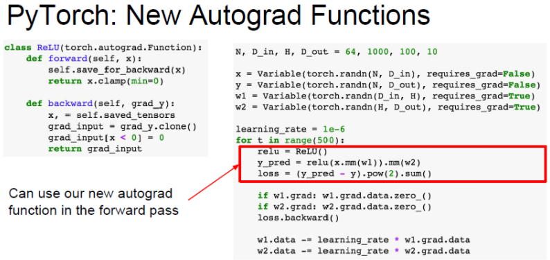
Example Define New Autograd function
PyTorch는 사용자에 목적에 맞는 새로운 Autograd Function을 정의할 수 있습니다.
대부분 이런 함수들이 이미 구현되어 있으므로 우리는 필요와 목적에 맞는 함수를 불러오면 됩니다.
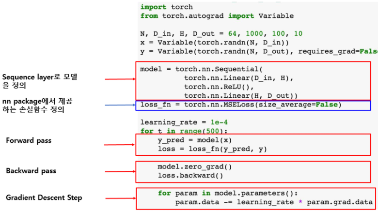
Example two Layer with PyTorch nn
PyTorch에서는 Higher level API를 nn Package가 담당합니다.
아래는 nn Package를 이용하여 Sequence layer로 model를 구현하는 방법을 보여줍니다.
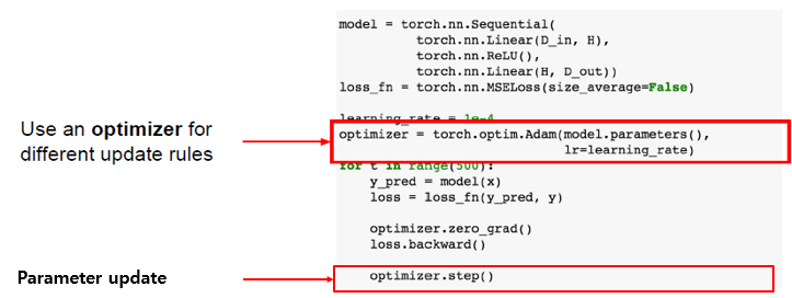
Example Optimizer
또한 PyTorch는 Optimizer operation을 제공합니다.
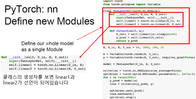
Example Define new Modules
nn module은 일종의 네트워크 레이어라고 생각하시면 됩니다.
이 모듈은 다른 모듈이 포함될 수도 있고 학습 가능한 가중치도 포함될 수 있습니다.
아래 코드는 2-Layer Net을 하나의 모듈로 정의한 코드입니다.
먼저 TwoLayerNet의 __init__생성자를 보시면 2개의 linear1과 linear2가 선언되어 있습니다.
두 개의 object를 클래스 안에 저장하고 있는 것 입니다. 마치 자식 module를 2개 저장하는 것과 같습니다.
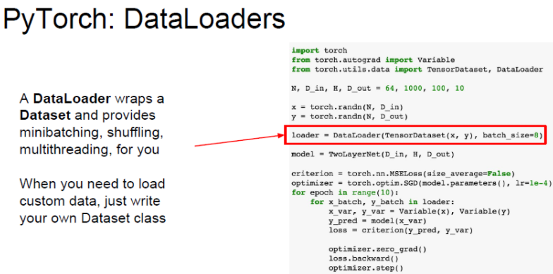
Example DataLoaders
PyTorch는 DataLoader를 제공합니다. DataLoader는 mini-batch를 관리해줍니다.
학습 도중에 Disk에서 mini-batch를 가져오는 작업을 알아서 관리해줍니다.
dataloader는 dataset를 wrapping 하는 일종의 추상화 객체를 제공해줍니다.
여기서 for문에 epoch는 전체 training dataset을 총 몇 번 반복할지를 말합니다.
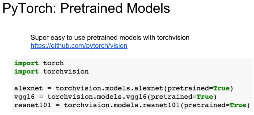
Example Pretrained Models
아래와 같이 torchvision이라는 라이브러리를 이용하면 alexnet, vgg, resnet등의 pre-trained model를 간편하게 다운받을 수 있습니다.
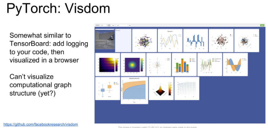
Example Visualization
visdom은 tensorflow의 tensorboard와 유사합니다.
이는 나중에 다룰 기회가 있으면 더 다루도록 하겠습니다.
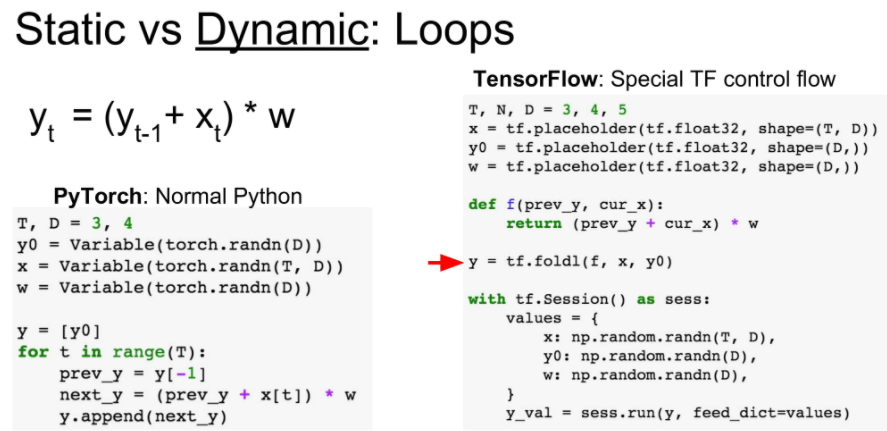
Static vs Dynamic Graphs
TensorFlow는 static graph, PyTorch는 dynamic Graph 라고 합니다.
- static graph : define & run
- dynamic graph : running time에 dynamic하게 graph를 바꿀 수 있습니다.
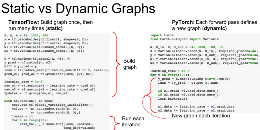
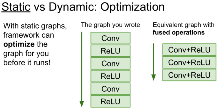
static graph의 큰 장점은 deep learing framework의 layer optimzer를 받을 수 있다는 것입니다.
compile 언어와 script 언어의 특징의 차이와 비슷하다.
아래 그림에서 이미 compile시 모델의 전체 구조를 알고 있으므로 Conv와 ReLU를 합친 fused operation으로 최적화 한 것을 볼 수 있습니다.
static graph는 한번 model이 정해진다면, build code 없이 model를 사용할 수 있다는 장점이 있습니다.
dynamic graph의 장점은 runtime에서 graph의 변형이 쉽다는 것입니다.
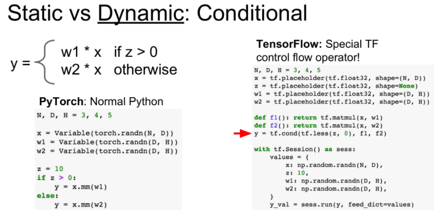
아래를 보시면 dynamic graph의 장점은 간단한 if 문으로 모델을 변경할 수 있습니다.
하지만 static graph는 이 모든 조건을 미리 graph에 넣어두어야 합니다.
또한 dynamic graph는 iteration의 강합니다.
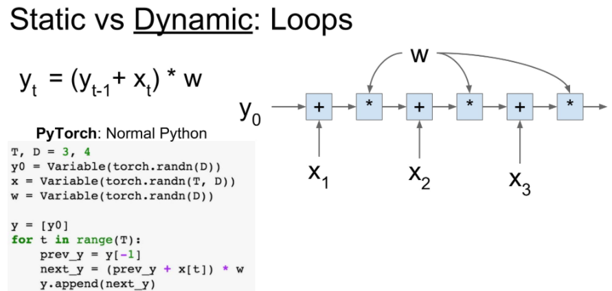
dynamic graph는 for문으로 로직을 짜는 것 같이 사용할 수 있지만,
static graph는 functional programming 처럼 미리 기능에 대한 선언을 함수로 해두어야 합니다.
아래 오른쪽으로 보시면 f함수를 미리 선언 하여 사용하는 것을 볼 수 있습니다.
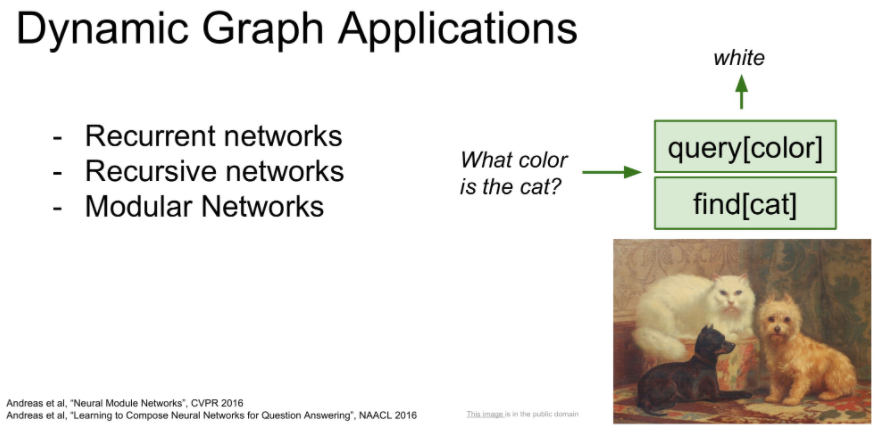
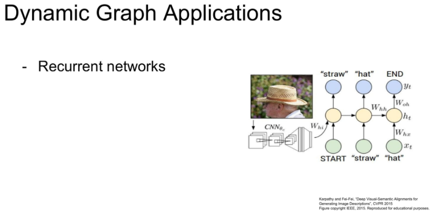
이러한 dynamic graph의 장점이 Recurrent networks를 구현하는데 유용하다고 합니다.
또한 module로 구성된 network를 유동적으로 컨트롤 할 수 있다는 장점이 있습니다.