1. Introduction

1-1 Difficulty of Mean-field Approach*

• assumes that all variables of the model(data, latent, parameters) are independent (but they are not!)
• simplifies the calculation, but can have poor approximations for complex models with dependent variables, which requires solving intractable expectations

*mean-field approach?
👉 commonly used method in VB for choosing the form of the approximate posterior

1-2 Auto-Encoding Variational Bayes (AEVB)

• in order to overcome such intractability, the paper suggests new algorithm called AEVB
• enables efficient, differentiable, and unbiased estimation of the variational lower bound via Stochastic Gradient Variational Bayes (SGVB) estimator
• simplifies posterior inference and model learning, avoiding costly iterative schemes like MCMC.

2. Method

2-1 Problem Scenario

Assumptions

• value $z^{(i)}$ generated from prior distribution $p_{\theta^{*}}(z)$ <- prior
• value $x^{(i)}$ generated from conditional distribution $p_{\theta^{*}}(x|z)$ <- likelihood
• PDF of prior & likelihood distribution are differentiable almost everywhere w.r.t. $\theta$ and z
• true parameters and latent variables are unknown
• do not simplify the marginal / posterior probabilities

Main Contributions

1. Efficient approximate ML or MAP estimation for the parameters $\theta$
2. Efficient approximate posterior inference of the latent variable z given an observed value x for a choice of parameters $\theta$
3. Efficient approximate marginal inference of the variable x

2-2 Variational Bound

1. Let marginal likelihood*
   $\log p_{\theta}(x^{(i)}) =D_{KL}(q_{\phi}(z|x^{(i)})||p_{\theta}(z|x^{(i)}))+\mathcal{L}(\theta, \phi;x^{(i)})$

2. Since the value of KL-Divergence is always non-negative,
   $\mathcal{L}(\theta, \phi;x^{(i)})$ becomes the lower bound.

3. Lower bound on the marginal likelihood of datapoint i can be re-written as :
   $\mathcal{L}(\theta,\phi;x^{(i)})=-D_{KL}(q_{\phi}(z|x^{(i)})||p_{\theta}(z))+\mathbb{E}_{q_{\phi}(z|x^{(i)})}[logp_{\theta}(x^{(i)}|z)]$

Gradient of the lower bound w.r.t. $\phi$, can lead to gradient estimator exhibiting high variance, thus impractical!
==> Importance of SGVB estimator

*marginal likelihood (evidence)?
👉 represents the probability of the observed data given the prior distribution of the model parameters

👉 When optimizing, since the marginal likelihood can make the computation intractable, we use variational lower bound.

2-3 Reparametrization Trick

• Let z be a continuous random variable, $z \sim q_{\phi}(z|x)$ be some conditional distribution.

• Then z can be expressed as:
  $z=g_{\phi}(\epsilon, x)$, where $\epsilon$ is a random variable following simple, known distribution

• $\int q_{\phi}(z|x)f(z)dz=\int p(\epsilon)f(z)d\epsilon=\int p(\epsilon)f(g_{\phi}(\epsilon,x))d\epsilon$

  • $\int q_{\phi}(z|x)f(z)dz$ :
    • an expectation of a function f(z) under the distribution $q_{\phi}(z|x)$, represented by the integral of f(z) times the PDF of z ($q_{\phi}(z|x)$), over all possible values of z
  • $\int p(\epsilon)f(z)d\epsilon$ :
    • changing the random variable of interest in the expectation calculation from z to $\epsilon$, which follows the distribution $q_{\phi}(z|x)$ and $p(\epsilon)$ respectively.
    • Since $\epsilon$ does not depend on the parameters $\phi$, it is possible to compute the gradient of the expectation w.r.t. $\phi$

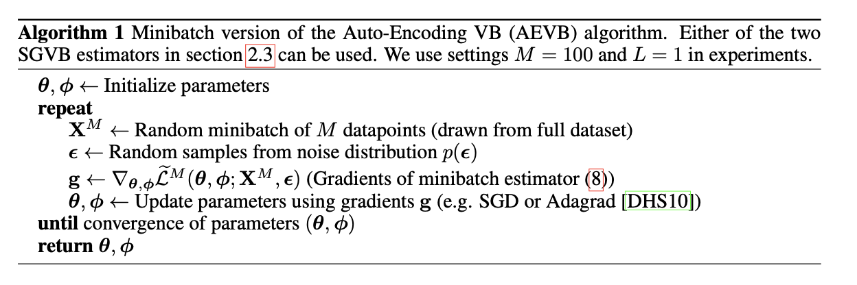
2-4 SGVB estimator and AEVB algorithm

1. After applying reparametrization trick of section 2-3, estimates of expectation of some function $f(z)$ w.r.t. $q_{\phi}(z|x)$ can be formed as :

   $\mathbb{E}_{q_{\phi}(z|x^{(i)})}[f(z)]=\mathbb{E}_{p(\epsilon)}[f(g_{\phi}(\epsilon,x^{(i)}))]\simeq \frac{1}{L}\Sigma^{L}_{l=1}f(g_{\phi}(\epsilon^{(l)},x^{(i)}))$
   

2. Yield generic Stochastic Gradient Variational Bayes estimator by applying technique in 1.

   $\tilde{\mathbb{L}}^{A}(\theta,\phi;x^{(i)})=\frac{1}{L}\Sigma ^{L}_{l=1}\log p_{\theta}(x^{(i)},z^{(i,l)})-\log q_{\phi}(z^{(i,l)}|x^{(i)})$

   where $z^{(i,l)}=g_{\phi}(\epsilon^{(i,l)}, x^{(i)})$ and $\epsilon^{(l)}\sim p(\epsilon)$

Below is the AEVB algorithm that utilizes above estimator.

3. Example : VAE

3-1 Variational approximate posterior

$\log q_{\phi}(z|x^{(i)})=\log \mathcal{N} (z;\mu^{(i)},\sigma^{2(i)}I)$

• mean and s.d. of approximate posterior $\mu^{(i)},\sigma^{2(i)}$ : parameters learned from encoder
• $\phi$ : variational parameters
• the main goal of VAE is to find good approximate posterior $\log q_{\phi}(z|x^{(i)})$ over the latent variables

3-2 Estimator for VAE and datapoint $x^{(i)}$

$\mathcal{L}(\theta,\phi;x^{(i)})\simeq \frac{1}{2}\Sigma^{J}_{j=1}(1+\log ((\sigma_{j}^{(i)})^2)-(\mu_{j}^{(i)})^2-(\sigma_{j}^{(i)})^2)+\frac{1}{L}\Sigma^{L}_{l=1}\log p_{\theta}(x^{(i)}|z^{(i,l)})$

where $z^{(i,l)}=\mu^{(i)}+\sigma^{(i)}\odot \epsilon^{(l)}$ and $\epsilon^{(l)}\sim\mathcal{N}(0,\mathbf{I})$

3-3 Architecture

Auto-encoder vs Variational Auto Encoder

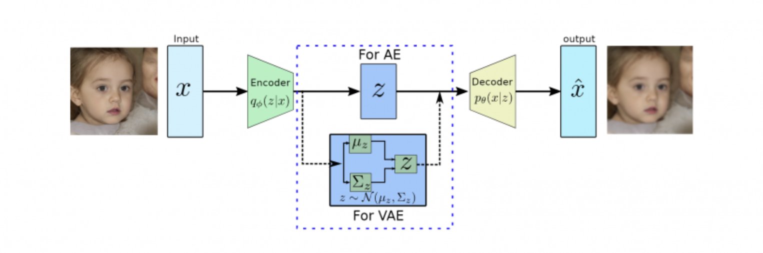
Source : https://data-science-blog.com/blog/2022/04/19/variational-autoencoders/

4. Conclusion

• SGVB is a novel estimator of the variational lower bound, resolving intractibility when parameters are optimized
• Since SGVB is differentiable and can be optimized straight forward, it can lead to efficient approximate inference with continuous latent variables.
• For the case of i.i.d. datasets and continuous latent variables per datapoint we introduce an efficient algorithm called Auto-Encoding VB (AEVB), learning an approximate inference model using the SGVB estimator.