새싹 인공지능 응용sw 개발자 양성 교육 프로그램 심선조 강사님 수업 정리 글입니다.
목차
1. 나만의 데이터 만들기
2. 데이터 저장 방법
3. 엑셀파일
4. 그래프 그리기
5. matplotlib 라이브러리 자유자재로 사용하기
6. 분석하기 좋은 데이터
7. 누락값처리
1. 나만의 데이터 만들기
df = pd.read_csv('data/scientists.csv')
df['Age'].max()
>>90
df['Age'] #'Age'만 뽑음
>>0 37
1 61
2 90
3 66
4 56
5 45
6 41
7 77
Name: Age, dtype: int64
df['Age'].mean() #age의 평균
>>59.125
df['Age']>df['Age'].mean() #비교연산자라 결과가 true or false로 반환
>>0 False
1 True
2 True
3 True
4 False
5 False
6 False
7 True
Name: Age, dtype: bool
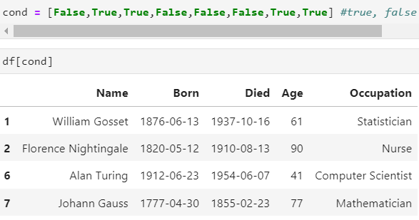
cond = [False,True,True,False,False,False,True,True] #true, false에 따른 조건에 맞는 것만 추출이 가능하다.
df[cond]
#df['Occupation'].get('Chemist') #occupation의 chemist만 추출해라
df['Occupation']=='Chemist' #조건부터 만들기
>>0 True
1 True
2 True
3 True
4 True
5 True
6 True
7 True
Name: Occupation, dtype: bool
df['Age'] + 100
>>0 137
1 161
2 190
3 166
4 156
5 145
6 141
7 177
Name: Age, dtype: int64
df['Age'] + pd.Series([1, 100]) #series로 데이터를 만든다. 데이터 갯수는 2개다.
#boradcasing 조건 = 스칼라, 같거나, 1이거나 age값은 8개인데 뒤에 데이터 값은 2개라서
#2개만 계산이 되고 nan로 처리가 된다. 오류가 나지는 않지만 nan계산이 된다.
>>0 38.0
1 161.0
2 NaN
3 NaN
4 NaN
5 NaN
6 NaN
7 NaN
dtype: float64
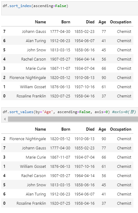
df['Age'].sort_index(ascending=False) #ascending=False 내림차순 정렬
>>7 77
6 41
5 45
4 56
3 66
2 90
1 61
0 37
Name: Age, dtype: int64

시리즈와 데이터프레임의 데이터 처리
- 열의 자료형 바꾸기와 새로운 열 추가하기
df.info() #dtype, object, int로 구성되어 있다.
>><class 'pandas.core.frame.DataFrame'>
RangeIndex: 8 entries, 0 to 7
Data columns (total 5 columns):
 #   Column      Non-Null Count  Dtype
---  ------      --------------  -----
 0   Name        8 non-null      object
 1   Born        8 non-null      object
 2   Died        8 non-null      object
 3   Age         8 non-null      int64
 4   Occupation  8 non-null      object
dtypes: int64(1), object(4)
memory usage: 448.0+ bytes
format
1999-09-09요런 형식
'%y-%m-%m'
pd.to_datetime = 날짜형으로 , numeric = 숫자형으로, timedelta = 날짜 간격을 줄 때
pd.to_datetime(df['Born']) #형태가 다르면 foramt을 바꿔줘야 한다. 0 1920-07-25
1 1876-06-13
2 1820-05-12
3 1867-11-07
4 1907-05-27
5 1813-03-15
6 1912-06-23
7 1777-04-30
Name: Born, dtype: datetime64[ns]df['Born_dt'] = pd.to_datetime(df['Born'],format='%Y-%m-%d')
df['Died_dt'] = pd.to_datetime(df['Died'],format='%Y-%m-%d')df.columnsIndex(['Name', 'Born', 'Died', 'Age', 'Occupation', 'Born_dt', 'Died_dt'], dtype='object')df.head(2)| Name | Born | Died | Age | Occupation | Born_dt | Died_dt | |
|---|---|---|---|---|---|---|---|
| 0 | Rosaline Franklin | 1920-07-25 | 1958-04-16 | 37 | Chemist | 1920-07-25 | 1958-04-16 |
| 1 | William Gosset | 1876-06-13 | 1937-10-16 | 61 | Statistician | 1876-06-13 | 1937-10-16 |
df['Died_dt']-df['Born_dt']0 13779 days
1 22404 days
2 32964 days
3 24345 days
4 20777 days
5 16529 days
6 15324 days
7 28422 days
dtype: timedelta64[ns]import randomrandom.seed(42) #random.seed()='무작위'의 결과를 특정한 값으로 고정
df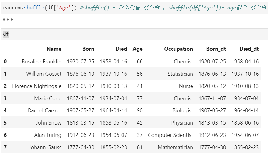
>>> df.columns
Index(['Name', 'Born', 'Died', 'Age', 'Occupation', 'Born_dt', 'Died_dt'], dtype='object')

df.drop(columns='Age',implace=True) #implace=True - 원본에 바로 적용 또는
#df or df1 =df.drop(columns='Age',implace=True) 이런 방법이 있다.
#'age'는 열이기때문에 axis=1을 줘야 한다. 그래서 index나 column에서 작업하는 것이 편하다.

2. 데이터 저장 방법
피클로 저장하기 = to_pickle 매서드 사용 csv(,), tsv(tab)
json: javascript object, text기반-> 메모장에서도 데이터를 볼 수 있다.
pickle과 json 데이터 저장 방법은 동일하다
txt기반 -> 메모장에서 볼 수 있음
byte기반 -> 메모장에서 볼 수 없지만 이미지, 동영상 그대로 저장 가능
pickled.dump(s) = 저장, pickled.load(s) = 읽기, s의 차이는 s가 안 붙으면 파일로 되어 있는 것을 불러올 떄는 s안 붙이고, 파일형태가 아니면 s를 사용한다.
>>>import pickle

>>>f = open('data.pickle', 'wb') #open() 파일 열어주는 것, 'w'= write, 'wb' = >>>write + byte라서
>>>pickle.dump(df,f)
>>>f.close() #파일객체는 close하는 것이 좋다.

>>>f = open('data.pickle', 'wb') #open() 파일 열어주는 것, 'w'= write, 'wb' = >>>write + byte라서
>>>pickle.dump(df,f)
>>>f.close() #파일객체는 close하는 것이 좋다.
pandas 사용하는 방법 to_pickle('파일명') read_pickle('파일명')
-> pandas에서 제공하는 df만 저장가능 opne안 해도 됨
import pickle df뿐만 아닌 다양한 형태 딕셔너리, 클래스 등등 오픈 가능
>>> df['Name'].to_list() #series는 list로 가능
['Rosaline Franklin',
 'William Gosset',
 'Florence Nightingale',
 'Marie Curie',
 'Rachel Carson',
 'John Snow',
 'Alan Turing',
 'Johann Gauss']

import json

>>>f = open('data.json','w') #json은 기본적으로 text형태다 그래서 바로df형태로 저장이 안 된다. to_json 사용하면 바로 변환가능
>>>json.dump(df['Name'].to_list(), f)
>>>f.close()

>>>f = open('data.json','r') #json은 기본적으로 text형태다 그래서 바로df형태로 저장이 안 된다. to_json 사용하면 바로 변환가능
>>>data = json.load(f)
>>>f.close()

>>>data
['Rosaline Franklin',
 'William Gosset',
 'Florence Nightingale',
 'Marie Curie',
 'Rachel Carson',
 'John Snow',
 'Alan Turing',
 'Johann Gauss']
3. 엑셀파일
!pip install xlwt #입력값을 넣는 것은 안 된다.
import xlwt #기본으로 설치 안 되어 있음, 최근 형태는 가능하지만 옛날 형태는 설치해서 사용해야 한다.
import openpyxl #기본으로 설치 됨

df.to_excel('df_excel.xls') #메세지는 뜨지만 저장은 된다.
df.to_excel('df_excel.xlsx')#기본처리가 되어있음
pd.read_excel()
4. 그래프 그리기
- 앤스콤 4분할 그래프 살펴보기
데이터 시각화가 좋은 이유는 그림을 보고 보기 좋게 한 눈에 들어온다.
데이터 집합은 4개의 그룹으로 구성, 4개의 데이터 그룹은 가각 평균, 분산과 같은 수칫값이나 상관관계, 회귀선이 같다는 특징.
4개 데이터 들은 다 다른데 대표값은 다 같다. 이 결과만 보고는 4개의 데이터가 같을 것이라고 착각할 수 있다.
요즘은 데이터사우루스 사용
- 데이터 분석 목적에 맞는 데이터를 모아 새로운 표(table)를 만들어야 한다.
- 측정한 값은 행(row)로 구성
- 변수는 열(column)로 구성
import seaborn as snsdf = sns.load_dataset('anscombe')type(df)pandas.core.frame.DataFramedf['dataset'].unique() #안에 몇 개 들어있는 지 확인하려면, unique사용해서 유일값을 추출하기array(['I', 'II', 'III', 'IV'], dtype=object)dataset1 = df[df['dataset']=='I'] #dataset의 I값을 dataset에 저장하기
dataset2 = df[df['dataset']=='II']
dataset3 = df[df['dataset']=='III']
dataset4 = df[df['dataset']=='IV']
dataset3| dataset | x | y | |
|---|---|---|---|
| 22 | III | 10.0 | 7.46 |
| 23 | III | 8.0 | 6.77 |
| 24 | III | 13.0 | 12.74 |
| 25 | III | 9.0 | 7.11 |
| 26 | III | 11.0 | 7.81 |
| 27 | III | 14.0 | 8.84 |
| 28 | III | 6.0 | 6.08 |
| 29 | III | 4.0 | 5.39 |
| 30 | III | 12.0 | 8.15 |
| 31 | III | 7.0 | 6.42 |
| 32 | III | 5.0 | 5.73 |
import matplotlib.pyplot as plt
plt.plot(dataset1['x'],dataset1['y'])[<matplotlib.lines.Line2D at 0x230e89f4af0>]
plt.plot(dataset1['x'],dataset1['y'],'o')[<matplotlib.lines.Line2D at 0x230e8a61fa0>]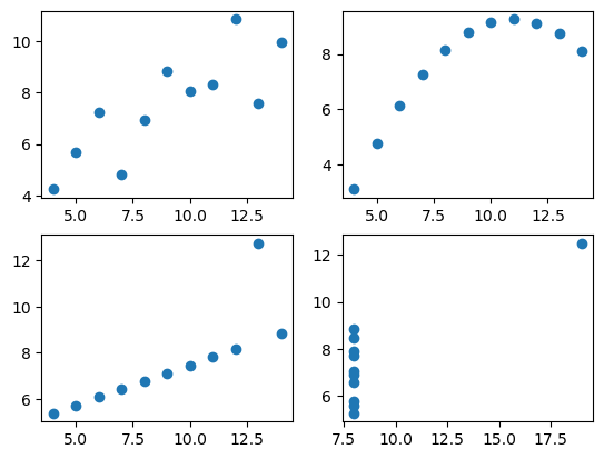
# 4개를 한 번에 그래프 그리기
fig = plt.figure()
a1 = fig.add_subplot(2,2,1) #2행의 2열의 1번째 꺼다
a2 = fig.add_subplot(2,2,2)
a3 = fig.add_subplot(2,2,3)
a4 = fig.add_subplot(2,2,4)
a1.plot(dataset1['x'],dataset1['y'],'o') #데이터 분포가 다 다르다
a2.plot(dataset2['x'],dataset2['y'],'o')
a3.plot(dataset3['x'],dataset3['y'],'o')
a4.plot(dataset4['x'],dataset4['y'],'o')[<matplotlib.lines.Line2D at 0x230ea0a9b50>]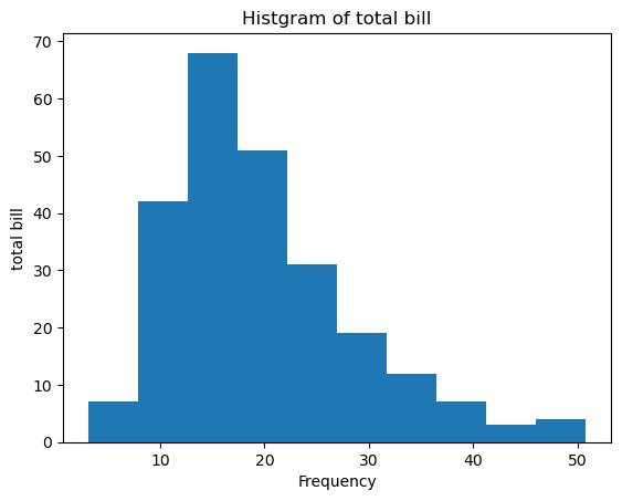
dataset1.mean()C:\Users\user\AppData\Local\Temp\ipykernel_11076\148656524.py:1: FutureWarning: Dropping of nuisance columns in DataFrame reductions (with 'numeric_only=None') is deprecated; in a future version this will raise TypeError. Select only valid columns before calling the reduction.
dataset1.mean()
x 9.000000
y 7.500909
dtype: float64dataset2.mean()C:\Users\user\AppData\Local\Temp\ipykernel_11076\3349088152.py:1: FutureWarning: Dropping of nuisance columns in DataFrame reductions (with 'numeric_only=None') is deprecated; in a future version this will raise TypeError. Select only valid columns before calling the reduction.
dataset2.mean()
x 9.000000
y 7.500909
dtype: float64dataset3.mean()C:\Users\user\AppData\Local\Temp\ipykernel_11076\2152253674.py:1: FutureWarning: Dropping of nuisance columns in DataFrame reductions (with 'numeric_only=None') is deprecated; in a future version this will raise TypeError. Select only valid columns before calling the reduction.
dataset3.mean()
x 9.0
y 7.5
dtype: float64dataset4.mean()C:\Users\user\AppData\Local\Temp\ipykernel_11076\1693280217.py:1: FutureWarning: Dropping of nuisance columns in DataFrame reductions (with 'numeric_only=None') is deprecated; in a future version this will raise TypeError. Select only valid columns before calling the reduction.
dataset4.mean()
x 9.000000
y 7.500909
dtype: float64dataset1.std() #표준편차C:\Users\user\AppData\Local\Temp\ipykernel_11076\45964655.py:1: FutureWarning: Dropping of nuisance columns in DataFrame reductions (with 'numeric_only=None') is deprecated; in a future version this will raise TypeError. Select only valid columns before calling the reduction.
dataset1.std() #표준편차
x 3.316625
y 2.031568
dtype: float64dataset1.corr() #상관계수| x | y | |
|---|---|---|
| x | 1.000000 | 0.816421 |
| y | 0.816421 | 1.000000 |
- 시각화를 하는 이유
통계와 시각화가 다를 수 있기 떄문에
5. matplotlib 라이브러리 자유자재로 사용하기
- 기초그래프 그리기
seaborn 라이브러리에는 tips라는 데이터 집합이 있다.
tips = sns.load_dataset('tips') #데이터 가져오면 데이터 상태 확인(head,sample,tail,info) 해야 한다
tips.head(2)| total_bill | tip | sex | smoker | day | time | size | |
|---|---|---|---|---|---|---|---|
| 0 | 16.99 | 1.01 | Female | No | Sun | Dinner | 2 |
| 1 | 10.34 | 1.66 | Male | No | Sun | Dinner | 3 |
tips.info() #244 non-null -> null값이 없다로 해석 가능<class 'pandas.core.frame.DataFrame'>
RangeIndex: 244 entries, 0 to 243
Data columns (total 7 columns):
# Column Non-Null Count Dtype
--- ------ -------------- -----
0 total_bill 244 non-null float64
1 tip 244 non-null float64
2 sex 244 non-null category
3 smoker 244 non-null category
4 day 244 non-null category
5 time 244 non-null category
6 size 244 non-null int64
dtypes: category(4), float64(2), int64(1)
memory usage: 7.4 KB- 기초 그래프 - 히스토그램, 산점도 그래프, 박스 그래프
히스토그램
히스토그램은 데이터프레임의 열 데이터 분포와 빈도를 살펴보는 요도로 사용하는 그래프
'일변량 그래프'라고 한다.
변수 하나만 있으면 된다.
값의 범위를 10개 범위로 나눠주고
해당 범위에 count를 해서
변수는 하나가 필요하고 데이터는 연속적인 값이 필요하다.
예를 들어 0~10까지 범위에 데이터 갯수가 몇 개가 있느냐
fig = plt.figure()
a1 = fig.add_subplot(1,1,1) #plt 은 기본 선 그래프
a1.hist(tips['total_bill'])  #his = 히스토그램, 데이터는 하나이다. 히스토그래은 모든 데이터를 그릴 수 잇는 것은 아니다. 어떤 구간에 데이터가 몰려 있는지 확인할 때 사용한다.
a1.set_title('Histgram of total bill') #그래프 제목
a1.set_xlabel('Frequency') #한글은 깨진다. 나중에 설정하는 법 배운다.
a1.set_ylabel('total bill')
Text(0, 0.5, 'total bill')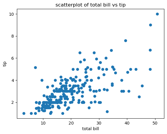
산전도 그래프
변수 2개 필요
값 2개의 관계, 값의 분포 확인할 때 사용한다.
fig1 = plt.figure()
a1 = fig1.add_subplot(1,1,1)
a1.scatter(tips['total_bill'], tips['tip']) # a1.scatter(tips[x축값], tips[y축값])
a1.set_title('scatterplot of total bill vs tip')
a1.set_xlabel('total bill')
a1.set_ylabel('tip')
Text(0, 0.5, 'tip')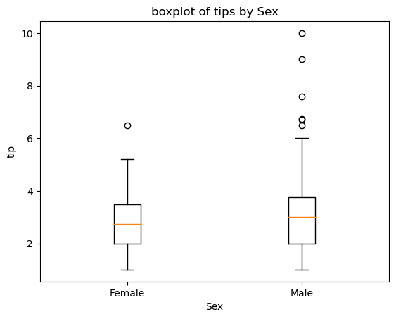
boxplot
이산형 변수와 연속형 변수를 함께 사용하는 그래프이다.
이산형 변수는 연결되지 않고 딱딱 끊어지는 것이다, 성별같이 명확하게 구분되는 값
연속형 변수는 tip과 같이 명확하게 셀 수 없는 범위의 값을 의미한다.
성별에 따른 tip의 분포를 본다.
fig2 = plt.figure()
a1 = fig2.add_subplot(1,1,1)
a1.boxplot([tips[tips['sex'] == 'Female']['tip'],
           tips[tips['sex'] == 'Male']['tip']],
          labels=['Female','Male']) #tips[tips['sex'] == 'Female']] tips = 컬럼이 여러개,tips[tips['sex'] == 'Female']['tips']함으로써 컬럼을 정해주는 것?
a1.set_title('boxplot of tips by Sex') #사용하는 값은 x값이지만 성별로 분류해서 넣어줘야 한다?
a1.set_xlabel('Sex')
a1.set_ylabel('tip')
Text(0, 0.5, 'tip')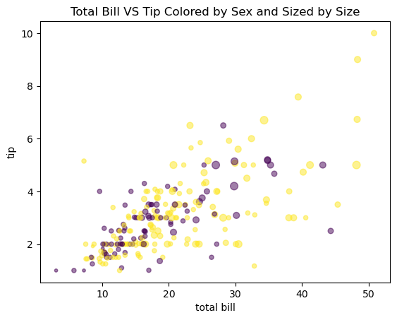
다변량 그래프
변수 3개 이상 사용한 그래프
산점도 그래프
def recode_sex(sex):
    if sex == 'Female':
        return 0
    else:
return 1 #return 함수가 종료되고 그 값을 함수 밖으로 보내준다. tips['sex_color']=tips['sex'].apply(recode_sex) tips
| total_bill | tip | sex | smoker | day | time | size | sex_color | |
|---|---|---|---|---|---|---|---|---|
| 0 | 16.99 | 1.01 | Female | No | Sun | Dinner | 2 | 0 |
| 1 | 10.34 | 1.66 | Male | No | Sun | Dinner | 3 | 1 |
| 2 | 21.01 | 3.50 | Male | No | Sun | Dinner | 3 | 1 |
| 3 | 23.68 | 3.31 | Male | No | Sun | Dinner | 2 | 1 |
| 4 | 24.59 | 3.61 | Female | No | Sun | Dinner | 4 | 0 |
| ... | ... | ... | ... | ... | ... | ... | ... | ... |
| 239 | 29.03 | 5.92 | Male | No | Sat | Dinner | 3 | 1 |
| 240 | 27.18 | 2.00 | Female | Yes | Sat | Dinner | 2 | 0 |
| 241 | 22.67 | 2.00 | Male | Yes | Sat | Dinner | 2 | 1 |
| 242 | 17.82 | 1.75 | Male | No | Sat | Dinner | 2 | 1 |
| 243 | 18.78 | 3.00 | Female | No | Thur | Dinner | 2 | 0 |
244 rows × 8 columns
fig3 = plt.figure()
a1 = fig3.add_subplot(1,1,1)
a1.scatter(tips['total_bill'], #,하고 엔터하면 줄을 바꿀 수 있다.
           tips['tip'],
           s=tips['size']*10, c=tips['sex_color'],
           alpha=0.5) # a1.scatter(tips[x축값], tips[y축값])
a1.set_title('Total Bill VS Tip Colored by Sex and Sized by Size')
a1.set_xlabel('total bill')
a1.set_ylabel('tip') #4개의 정보가 들어갔다
Text(0, 0.5, 'tip')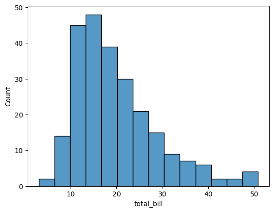
- seaborn 라이브러리 자유자재로 사용하기
sns.histplot(tips['total_bill'])<AxesSubplot:xlabel='total_bill', ylabel='Count'>
ax = plt.subplots()
ax = sns.histplot(tips['total_bill'],kde=True) #kde=True 밀집도 그래프 on
ax.set_title('total bill histgram')
Text(0.5, 1.0, 'total bill histgram')
- countplot
히스토그램과 비슷
히스토그램은 연속값의 범위를 나눠서 갯수를 그래프로 나눔
카운트플롯은 이상값을 이용
ax = plt.subplot()
ax = sns.histplot(data=tips,x='total_bill',kde=True)
ax.set_title('totla bill histogram')
Text(0.5, 1.0, 'totla bill histogram')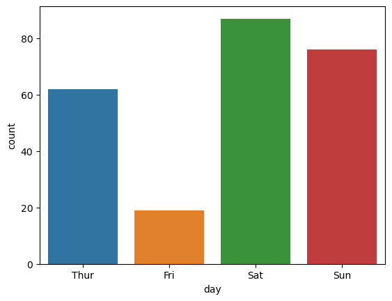
sns.countplot(data=tips,x='day')<AxesSubplot:xlabel='day', ylabel='count'>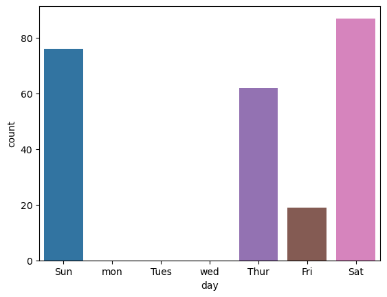
tips['day'].unique()['Sun', 'Sat', 'Thur', 'Fri']
Categories (4, object): ['Thur', 'Fri', 'Sat', 'Sun']day_list = ['Sun', 'mon', 'Tues', 'wed', 'Thur', 'Fri', 'Sat'] #원하는 순서대로 바꾸는 방법sns.countplot(data=tips,x='day',order=day_list)<AxesSubplot:xlabel='day', ylabel='count'>#요즘은 seaborn을 많이 쓴다, 플론다이닝은 r에서 넘어온 사람이 많이 쓴다.
6 분석하기 좋은 데이터
깔끔한 데이터 = tidy data, 클렌징 작업
- 데이터 분석 목적에 맞는 데이터를 모아 새로운 표(table)를 만들어야 한다.
- 측정한 값은 행(row)로 구성
- 변수는 열(column)로 구성
데이터 연결
- concat메서드로 데이터 연결하기
import pandas as pddf1 = pd.read_csv('data/concat_1.csv')
df2 = pd.read_csv('data/concat_2.csv')
df3 = pd.read_csv('data/concat_3.csv')df1| A | B | C | D | |
|---|---|---|---|---|
| 0 | a0 | b0 | c0 | d0 |
| 1 | a1 | b1 | c1 | d1 |
| 2 | a2 | b2 | c2 | d2 |
| 3 | a3 | b3 | c3 | d3 |
df2| A | B | C | D | |
|---|---|---|---|---|
| 0 | a4 | b4 | c4 | d4 |
| 1 | a5 | b5 | c5 | d5 |
| 2 | a6 | b6 | c6 | d6 |
| 3 | a7 | b7 | c7 | d7 |
df3| A | B | C | D | |
|---|---|---|---|---|
| 0 | a8 | b8 | c8 | d8 |
| 1 | a9 | b9 | c9 | d9 |
| 2 | a10 | b10 | c10 | d10 |
| 3 | a11 | b11 | c11 | d11 |
pd.concat([df1, df2, df3]) | A | B | C | D | |
|---|---|---|---|---|
| 0 | a0 | b0 | c0 | d0 |
| 1 | a1 | b1 | c1 | d1 |
| 2 | a2 | b2 | c2 | d2 |
| 3 | a3 | b3 | c3 | d3 |
| 0 | a4 | b4 | c4 | d4 |
| 1 | a5 | b5 | c5 | d5 |
| 2 | a6 | b6 | c6 | d6 |
| 3 | a7 | b7 | c7 | d7 |
| 0 | a8 | b8 | c8 | d8 |
| 1 | a9 | b9 | c9 | d9 |
| 2 | a10 | b10 | c10 | d10 |
| 3 | a11 | b11 | c11 | d11 |
pd.concat(
objs: 'Iterable[NDFrame] | Mapping[Hashable, NDFrame]',
axis: 'Axis' = 0, #행단위라서 밑으로 붙는다, axis=1이면 옆으로 붙는다.
join: 'str' = 'outer', #inner join 키값이 동일하면 조인 outter조인은 키값 안 동일해서 조인 # a,b,c 같은 것 끼리 연결, 뒤에는 index가 같은 것 끼리 연결?
ignore_index: 'bool' = False,
keys=None,
levels=None,
names=None,
verify_integrity: 'bool' = False,
sort: 'bool' = False,
copy: 'bool' = True,
) -> 'DataFrame | Series'
pd.concat([df1, df2, df3],axis=1) | A | B | C | D | A | B | C | D | A | B | C | D | |
|---|---|---|---|---|---|---|---|---|---|---|---|---|
| 0 | a0 | b0 | c0 | d0 | a4 | b4 | c4 | d4 | a8 | b8 | c8 | d8 |
| 1 | a1 | b1 | c1 | d1 | a5 | b5 | c5 | d5 | a9 | b9 | c9 | d9 |
| 2 | a2 | b2 | c2 | d2 | a6 | b6 | c6 | d6 | a10 | b10 | c10 | d10 |
| 3 | a3 | b3 | c3 | d3 | a7 | b7 | c7 | d7 | a11 | b11 | c11 | d11 |
new = pd.Series(['n1','n2','n3','n4']) pd.concat([df1,new]) #outer join은 공통된 값이 없어도 연결해 준다.| A | B | C | D | 0 | |
|---|---|---|---|---|---|
| 0 | a0 | b0 | c0 | d0 | NaN |
| 1 | a1 | b1 | c1 | d1 | NaN |
| 2 | a2 | b2 | c2 | d2 | NaN |
| 3 | a3 | b3 | c3 | d3 | NaN |
| 0 | NaN | NaN | NaN | NaN | n1 |
| 1 | NaN | NaN | NaN | NaN | n2 |
| 2 | NaN | NaN | NaN | NaN | n3 |
| 3 | NaN | NaN | NaN | NaN | n4 |
pd.DataFrame([['n1','n2','n3','n4']]) #번호는 따로 지정 안 해서 일련번호로 붙는다| 0 | 1 | 2 | 3 | |
|---|---|---|---|---|
| 0 | n1 | n2 | n3 | n4 |
new_df = pd.DataFrame([['n1','n2','n3','n4']],columns=['A', 'B', 'C', 'D'])df1.columnsIndex(['A', 'B', 'C', 'D'], dtype='object')pd.concat([df1,new_df]) #sql의 join개념과 다르다. column이름 같은 것 끼리, | A | B | C | D | |
|---|---|---|---|---|
| 0 | a0 | b0 | c0 | d0 |
| 1 | a1 | b1 | c1 | d1 |
| 2 | a2 | b2 | c2 | d2 |
| 3 | a3 | b3 | c3 | d3 |
| 0 | n1 | n2 | n3 | n4 |
df1.append(new_df)C:\Users\user\AppData\Local\Temp\ipykernel_3844\1631729507.py:1: FutureWarning: The frame.append method is deprecated and will be removed from pandas in a future version. Use pandas.concat instead.
df1.append(new_df)| A | B | C | D | |
|---|---|---|---|---|
| 0 | a0 | b0 | c0 | d0 |
| 1 | a1 | b1 | c1 | d1 |
| 2 | a2 | b2 | c2 | d2 |
| 3 | a3 | b3 | c3 | d3 |
| 0 | n1 | n2 | n3 | n4 |
pd.concat([df1, df2, df3],axis=1) #index값이 0123이렇게 되어 있는데 기존에 있는 것 무시하고 새로 구현하려면| A | B | C | D | A | B | C | D | A | B | C | D | |
|---|---|---|---|---|---|---|---|---|---|---|---|---|
| 0 | a0 | b0 | c0 | d0 | a4 | b4 | c4 | d4 | a8 | b8 | c8 | d8 |
| 1 | a1 | b1 | c1 | d1 | a5 | b5 | c5 | d5 | a9 | b9 | c9 | d9 |
| 2 | a2 | b2 | c2 | d2 | a6 | b6 | c6 | d6 | a10 | b10 | c10 | d10 |
| 3 | a3 | b3 | c3 | d3 | a7 | b7 | c7 | d7 | a11 | b11 | c11 | d11 |
pd.concat([df1, df2, df3],axis=0,ignore_index=True)#index값이 0123이렇게 되어 있는데 기존에 있는 것 무시하고 새로 구현하려면 ignore사용| A | B | C | D | |
|---|---|---|---|---|
| 0 | a0 | b0 | c0 | d0 |
| 1 | a1 | b1 | c1 | d1 |
| 2 | a2 | b2 | c2 | d2 |
| 3 | a3 | b3 | c3 | d3 |
| 4 | a4 | b4 | c4 | d4 |
| 5 | a5 | b5 | c5 | d5 |
| 6 | a6 | b6 | c6 | d6 |
| 7 | a7 | b7 | c7 | d7 |
| 8 | a8 | b8 | c8 | d8 |
| 9 | a9 | b9 | c9 | d9 |
| 10 | a10 | b10 | c10 | d10 |
| 11 | a11 | b11 | c11 | d11 |
pd.concat([df1,new],join='inner') #inner로 하면 공통된 부분이 없어서 아무것도 안 나온다| 0 |
|---|
| 1 |
| 2 |
| 3 |
| 0 |
| 1 |
| 2 |
| 3 |
데이터 연결 마무리
- merge 메서드 사용하기
person = pd.read_csv('data/survey_person.csv')
site = pd.read_csv('data/survey_site.csv')
survey = pd.read_csv('data/survey_survey.csv')
visited = pd.read_csv('data/survey_visited.csv')
sub_visited = visited.loc[[0,2,6]] #index값이 0, 2, 6인 값만 가져와라?sub_visited| ident | site | dated | |
|---|---|---|---|
| 0 | 619 | DR-1 | 1927-02-08 |
| 2 | 734 | DR-3 | 1939-01-07 |
| 6 | 837 | MSK-4 | 1932-01-14 |
#pandas의 merger있고 dataframde의 merger가 있다
그냥 merge는 왼쪽 오른쪽
site.merge는 오른쪽만
pd.merge() -> dataframe이 2개가 들어가야 한다.
merge는 join과 비슷하다.
?left_on, right_on
#pd.merge()
site.merge(sub_visited,left_on='name',right_on='site')| name | lat | long | ident | site | dated | |
|---|---|---|---|---|---|---|
| 0 | DR-1 | -49.85 | -128.57 | 619 | DR-1 | 1927-02-08 |
| 1 | DR-3 | -47.15 | -126.72 | 734 | DR-3 | 1939-01-07 |
| 2 | MSK-4 | -48.87 | -123.40 | 837 | MSK-4 | 1932-01-14 |
concat - column과 index가 동일한 것 끼리 연결
merge - 데이터값끼리 동일한 것 끼리 연결, join
7. 누락값처리
- 누락값이란?
누락값은 NaN, NAN, nan 표기 가능
from numpy import NaN,NAN,nanNaN == TrueFalseNAN == FalseFalsenan == ''Falsenan == 0False#누락값 확인
pd.isna(nan)True#누락값 확인
pd.isnull(nan)Truepd.notnull(nan)False#누락값이 생기는 이유 - outerjoin할 때 생길 수 있다, 데이터 입력할 때 실수
#누락값의 개수 구하기
ebola = pd.read_csv('data/country_timeseries.csv')ebola
| Date | Day | Cases_Guinea | Cases_Liberia | Cases_SierraLeone | Cases_Nigeria | Cases_Senegal | Cases_UnitedStates | Cases_Spain | Cases_Mali | Deaths_Guinea | Deaths_Liberia | Deaths_SierraLeone | Deaths_Nigeria | Deaths_Senegal | Deaths_UnitedStates | Deaths_Spain | Deaths_Mali | |
|---|---|---|---|---|---|---|---|---|---|---|---|---|---|---|---|---|---|---|
| 0 | 1/5/2015 | 289 | 2776.0 | NaN | 10030.0 | NaN | NaN | NaN | NaN | NaN | 1786.0 | NaN | 2977.0 | NaN | NaN | NaN | NaN | NaN |
| 1 | 1/4/2015 | 288 | 2775.0 | NaN | 9780.0 | NaN | NaN | NaN | NaN | NaN | 1781.0 | NaN | 2943.0 | NaN | NaN | NaN | NaN | NaN |
| 2 | 1/3/2015 | 287 | 2769.0 | 8166.0 | 9722.0 | NaN | NaN | NaN | NaN | NaN | 1767.0 | 3496.0 | 2915.0 | NaN | NaN | NaN | NaN | NaN |
| 3 | 1/2/2015 | 286 | NaN | 8157.0 | NaN | NaN | NaN | NaN | NaN | NaN | NaN | 3496.0 | NaN | NaN | NaN | NaN | NaN | NaN |
| 4 | 12/31/2014 | 284 | 2730.0 | 8115.0 | 9633.0 | NaN | NaN | NaN | NaN | NaN | 1739.0 | 3471.0 | 2827.0 | NaN | NaN | NaN | NaN | NaN |
| ... | ... | ... | ... | ... | ... | ... | ... | ... | ... | ... | ... | ... | ... | ... | ... | ... | ... | ... |
| 117 | 3/27/2014 | 5 | 103.0 | 8.0 | 6.0 | NaN | NaN | NaN | NaN | NaN | 66.0 | 6.0 | 5.0 | NaN | NaN | NaN | NaN | NaN |
| 118 | 3/26/2014 | 4 | 86.0 | NaN | NaN | NaN | NaN | NaN | NaN | NaN | 62.0 | NaN | NaN | NaN | NaN | NaN | NaN | NaN |
| 119 | 3/25/2014 | 3 | 86.0 | NaN | NaN | NaN | NaN | NaN | NaN | NaN | 60.0 | NaN | NaN | NaN | NaN | NaN | NaN | NaN |
| 120 | 3/24/2014 | 2 | 86.0 | NaN | NaN | NaN | NaN | NaN | NaN | NaN | 59.0 | NaN | NaN | NaN | NaN | NaN | NaN | NaN |
| 121 | 3/22/2014 | 0 | 49.0 | NaN | NaN | NaN | NaN | NaN | NaN | NaN | 29.0 | NaN | NaN | NaN | NaN | NaN | NaN | NaN |
122 rows × 18 columns
ebola.head(3)| Date | Day | Cases_Guinea | Cases_Liberia | Cases_SierraLeone | Cases_Nigeria | Cases_Senegal | Cases_UnitedStates | Cases_Spain | Cases_Mali | Deaths_Guinea | Deaths_Liberia | Deaths_SierraLeone | Deaths_Nigeria | Deaths_Senegal | Deaths_UnitedStates | Deaths_Spain | Deaths_Mali | |
|---|---|---|---|---|---|---|---|---|---|---|---|---|---|---|---|---|---|---|
| 0 | 1/5/2015 | 289 | 2776.0 | NaN | 10030.0 | NaN | NaN | NaN | NaN | NaN | 1786.0 | NaN | 2977.0 | NaN | NaN | NaN | NaN | NaN |
| 1 | 1/4/2015 | 288 | 2775.0 | NaN | 9780.0 | NaN | NaN | NaN | NaN | NaN | 1781.0 | NaN | 2943.0 | NaN | NaN | NaN | NaN | NaN |
| 2 | 1/3/2015 | 287 | 2769.0 | 8166.0 | 9722.0 | NaN | NaN | NaN | NaN | NaN | 1767.0 | 3496.0 | 2915.0 | NaN | NaN | NaN | NaN | NaN |
ebola.tail(3)| Date | Day | Cases_Guinea | Cases_Liberia | Cases_SierraLeone | Cases_Nigeria | Cases_Senegal | Cases_UnitedStates | Cases_Spain | Cases_Mali | Deaths_Guinea | Deaths_Liberia | Deaths_SierraLeone | Deaths_Nigeria | Deaths_Senegal | Deaths_UnitedStates | Deaths_Spain | Deaths_Mali | |
|---|---|---|---|---|---|---|---|---|---|---|---|---|---|---|---|---|---|---|
| 119 | 3/25/2014 | 3 | 86.0 | NaN | NaN | NaN | NaN | NaN | NaN | NaN | 60.0 | NaN | NaN | NaN | NaN | NaN | NaN | NaN |
| 120 | 3/24/2014 | 2 | 86.0 | NaN | NaN | NaN | NaN | NaN | NaN | NaN | 59.0 | NaN | NaN | NaN | NaN | NaN | NaN | NaN |
| 121 | 3/22/2014 | 0 | 49.0 | NaN | NaN | NaN | NaN | NaN | NaN | NaN | 29.0 | NaN | NaN | NaN | NaN | NaN | NaN | NaN |
ebola.count() #nan값이 포함되면 결과는 nan이 되기 때문에 기본적으로 nan값은 빼고 계산되도록 해준다.Date 122
Day 122
Cases_Guinea 93
Cases_Liberia 83
Cases_SierraLeone 87
Cases_Nigeria 38
Cases_Senegal 25
Cases_UnitedStates 18
Cases_Spain 16
Cases_Mali 12
Deaths_Guinea 92
Deaths_Liberia 81
Deaths_SierraLeone 87
Deaths_Nigeria 38
Deaths_Senegal 22
Deaths_UnitedStates 18
Deaths_Spain 16
Deaths_Mali 12
dtype: int64#nan이 몇 개가 있는 지 확인
pd.isna(ebola).sum() # sum()= true인 것만 집계가 된다. nan= true이니까, nan의 개수가 출련된다.Date 0
Day 0
Cases_Guinea 29
Cases_Liberia 39
Cases_SierraLeone 35
Cases_Nigeria 84
Cases_Senegal 97
Cases_UnitedStates 104
Cases_Spain 106
Cases_Mali 110
Deaths_Guinea 30
Deaths_Liberia 41
Deaths_SierraLeone 35
Deaths_Nigeria 84
Deaths_Senegal 100
Deaths_UnitedStates 104
Deaths_Spain 106
Deaths_Mali 110
dtype: int64pd.isna(ebola).sum().sum() #총 개수 합계1214#value count - 해당하는 컬럽안의 유일값을 뽑는다. 그 유일값이 몇 번 반복됬는 지 알 수 있따.
#누락값 처리 - 변경, 삭제
ebola['Cases_Guinea'].value_counts()86.0 3
495.0 2
112.0 2
390.0 2
408.0 1
..
1199.0 1
1298.0 1
1350.0 1
1472.0 1
49.0 1
Name: Cases_Guinea, Length: 88, dtype: int64ebola.fillna(0) #dropna 빼는것, fillna 채우는것, 평균으로 채우는 경우도 있음, 누적되서 들어가면 0으로 채우면 안됨 -> 중간값, 앞 쪽데이터 값을 넣어줌| Date | Day | Cases_Guinea | Cases_Liberia | Cases_SierraLeone | Cases_Nigeria | Cases_Senegal | Cases_UnitedStates | Cases_Spain | Cases_Mali | Deaths_Guinea | Deaths_Liberia | Deaths_SierraLeone | Deaths_Nigeria | Deaths_Senegal | Deaths_UnitedStates | Deaths_Spain | Deaths_Mali | |
|---|---|---|---|---|---|---|---|---|---|---|---|---|---|---|---|---|---|---|
| 0 | 1/5/2015 | 289 | 2776.0 | 0.0 | 10030.0 | 0.0 | 0.0 | 0.0 | 0.0 | 0.0 | 1786.0 | 0.0 | 2977.0 | 0.0 | 0.0 | 0.0 | 0.0 | 0.0 |
| 1 | 1/4/2015 | 288 | 2775.0 | 0.0 | 9780.0 | 0.0 | 0.0 | 0.0 | 0.0 | 0.0 | 1781.0 | 0.0 | 2943.0 | 0.0 | 0.0 | 0.0 | 0.0 | 0.0 |
| 2 | 1/3/2015 | 287 | 2769.0 | 8166.0 | 9722.0 | 0.0 | 0.0 | 0.0 | 0.0 | 0.0 | 1767.0 | 3496.0 | 2915.0 | 0.0 | 0.0 | 0.0 | 0.0 | 0.0 |
| 3 | 1/2/2015 | 286 | 0.0 | 8157.0 | 0.0 | 0.0 | 0.0 | 0.0 | 0.0 | 0.0 | 0.0 | 3496.0 | 0.0 | 0.0 | 0.0 | 0.0 | 0.0 | 0.0 |
| 4 | 12/31/2014 | 284 | 2730.0 | 8115.0 | 9633.0 | 0.0 | 0.0 | 0.0 | 0.0 | 0.0 | 1739.0 | 3471.0 | 2827.0 | 0.0 | 0.0 | 0.0 | 0.0 | 0.0 |
| ... | ... | ... | ... | ... | ... | ... | ... | ... | ... | ... | ... | ... | ... | ... | ... | ... | ... | ... |
| 117 | 3/27/2014 | 5 | 103.0 | 8.0 | 6.0 | 0.0 | 0.0 | 0.0 | 0.0 | 0.0 | 66.0 | 6.0 | 5.0 | 0.0 | 0.0 | 0.0 | 0.0 | 0.0 |
| 118 | 3/26/2014 | 4 | 86.0 | 0.0 | 0.0 | 0.0 | 0.0 | 0.0 | 0.0 | 0.0 | 62.0 | 0.0 | 0.0 | 0.0 | 0.0 | 0.0 | 0.0 | 0.0 |
| 119 | 3/25/2014 | 3 | 86.0 | 0.0 | 0.0 | 0.0 | 0.0 | 0.0 | 0.0 | 0.0 | 60.0 | 0.0 | 0.0 | 0.0 | 0.0 | 0.0 | 0.0 | 0.0 |
| 120 | 3/24/2014 | 2 | 86.0 | 0.0 | 0.0 | 0.0 | 0.0 | 0.0 | 0.0 | 0.0 | 59.0 | 0.0 | 0.0 | 0.0 | 0.0 | 0.0 | 0.0 | 0.0 |
| 121 | 3/22/2014 | 0 | 49.0 | 0.0 | 0.0 | 0.0 | 0.0 | 0.0 | 0.0 | 0.0 | 29.0 | 0.0 | 0.0 | 0.0 | 0.0 | 0.0 | 0.0 | 0.0 |
122 rows × 18 columns
ebola.fillna(method='ffill') #nan유지 ,fillna 원본값은 그대로 두고 return값만 돌려준다 #ffill앞쪽값으로 채워졌다.| Date | Day | Cases_Guinea | Cases_Liberia | Cases_SierraLeone | Cases_Nigeria | Cases_Senegal | Cases_UnitedStates | Cases_Spain | Cases_Mali | Deaths_Guinea | Deaths_Liberia | Deaths_SierraLeone | Deaths_Nigeria | Deaths_Senegal | Deaths_UnitedStates | Deaths_Spain | Deaths_Mali | |
|---|---|---|---|---|---|---|---|---|---|---|---|---|---|---|---|---|---|---|
| 0 | 1/5/2015 | 289 | 2776.0 | NaN | 10030.0 | NaN | NaN | NaN | NaN | NaN | 1786.0 | NaN | 2977.0 | NaN | NaN | NaN | NaN | NaN |
| 1 | 1/4/2015 | 288 | 2775.0 | NaN | 9780.0 | NaN | NaN | NaN | NaN | NaN | 1781.0 | NaN | 2943.0 | NaN | NaN | NaN | NaN | NaN |
| 2 | 1/3/2015 | 287 | 2769.0 | 8166.0 | 9722.0 | NaN | NaN | NaN | NaN | NaN | 1767.0 | 3496.0 | 2915.0 | NaN | NaN | NaN | NaN | NaN |
| 3 | 1/2/2015 | 286 | 2769.0 | 8157.0 | 9722.0 | NaN | NaN | NaN | NaN | NaN | 1767.0 | 3496.0 | 2915.0 | NaN | NaN | NaN | NaN | NaN |
| 4 | 12/31/2014 | 284 | 2730.0 | 8115.0 | 9633.0 | NaN | NaN | NaN | NaN | NaN | 1739.0 | 3471.0 | 2827.0 | NaN | NaN | NaN | NaN | NaN |
| ... | ... | ... | ... | ... | ... | ... | ... | ... | ... | ... | ... | ... | ... | ... | ... | ... | ... | ... |
| 117 | 3/27/2014 | 5 | 103.0 | 8.0 | 6.0 | 0.0 | 1.0 | 1.0 | 1.0 | 1.0 | 66.0 | 6.0 | 5.0 | 0.0 | 0.0 | 0.0 | 1.0 | 1.0 |
| 118 | 3/26/2014 | 4 | 86.0 | 8.0 | 6.0 | 0.0 | 1.0 | 1.0 | 1.0 | 1.0 | 62.0 | 6.0 | 5.0 | 0.0 | 0.0 | 0.0 | 1.0 | 1.0 |
| 119 | 3/25/2014 | 3 | 86.0 | 8.0 | 6.0 | 0.0 | 1.0 | 1.0 | 1.0 | 1.0 | 60.0 | 6.0 | 5.0 | 0.0 | 0.0 | 0.0 | 1.0 | 1.0 |
| 120 | 3/24/2014 | 2 | 86.0 | 8.0 | 6.0 | 0.0 | 1.0 | 1.0 | 1.0 | 1.0 | 59.0 | 6.0 | 5.0 | 0.0 | 0.0 | 0.0 | 1.0 | 1.0 |
| 121 | 3/22/2014 | 0 | 49.0 | 8.0 | 6.0 | 0.0 | 1.0 | 1.0 | 1.0 | 1.0 | 29.0 | 6.0 | 5.0 | 0.0 | 0.0 | 0.0 | 1.0 | 1.0 |
122 rows × 18 columns
ebola #앞쪽값으로 채워졌다.| Date | Day | Cases_Guinea | Cases_Liberia | Cases_SierraLeone | Cases_Nigeria | Cases_Senegal | Cases_UnitedStates | Cases_Spain | Cases_Mali | Deaths_Guinea | Deaths_Liberia | Deaths_SierraLeone | Deaths_Nigeria | Deaths_Senegal | Deaths_UnitedStates | Deaths_Spain | Deaths_Mali | |
|---|---|---|---|---|---|---|---|---|---|---|---|---|---|---|---|---|---|---|
| 0 | 1/5/2015 | 289 | 2776.0 | NaN | 10030.0 | NaN | NaN | NaN | NaN | NaN | 1786.0 | NaN | 2977.0 | NaN | NaN | NaN | NaN | NaN |
| 1 | 1/4/2015 | 288 | 2775.0 | NaN | 9780.0 | NaN | NaN | NaN | NaN | NaN | 1781.0 | NaN | 2943.0 | NaN | NaN | NaN | NaN | NaN |
| 2 | 1/3/2015 | 287 | 2769.0 | 8166.0 | 9722.0 | NaN | NaN | NaN | NaN | NaN | 1767.0 | 3496.0 | 2915.0 | NaN | NaN | NaN | NaN | NaN |
| 3 | 1/2/2015 | 286 | NaN | 8157.0 | NaN | NaN | NaN | NaN | NaN | NaN | NaN | 3496.0 | NaN | NaN | NaN | NaN | NaN | NaN |
| 4 | 12/31/2014 | 284 | 2730.0 | 8115.0 | 9633.0 | NaN | NaN | NaN | NaN | NaN | 1739.0 | 3471.0 | 2827.0 | NaN | NaN | NaN | NaN | NaN |
| ... | ... | ... | ... | ... | ... | ... | ... | ... | ... | ... | ... | ... | ... | ... | ... | ... | ... | ... |
| 117 | 3/27/2014 | 5 | 103.0 | 8.0 | 6.0 | NaN | NaN | NaN | NaN | NaN | 66.0 | 6.0 | 5.0 | NaN | NaN | NaN | NaN | NaN |
| 118 | 3/26/2014 | 4 | 86.0 | NaN | NaN | NaN | NaN | NaN | NaN | NaN | 62.0 | NaN | NaN | NaN | NaN | NaN | NaN | NaN |
| 119 | 3/25/2014 | 3 | 86.0 | NaN | NaN | NaN | NaN | NaN | NaN | NaN | 60.0 | NaN | NaN | NaN | NaN | NaN | NaN | NaN |
| 120 | 3/24/2014 | 2 | 86.0 | NaN | NaN | NaN | NaN | NaN | NaN | NaN | 59.0 | NaN | NaN | NaN | NaN | NaN | NaN | NaN |
| 121 | 3/22/2014 | 0 | 49.0 | NaN | NaN | NaN | NaN | NaN | NaN | NaN | 29.0 | NaN | NaN | NaN | NaN | NaN | NaN | NaN |
122 rows × 18 columns
ebola.fillna(method='bfill') #뒤쪽값으로 채워졌다.| Date | Day | Cases_Guinea | Cases_Liberia | Cases_SierraLeone | Cases_Nigeria | Cases_Senegal | Cases_UnitedStates | Cases_Spain | Cases_Mali | Deaths_Guinea | Deaths_Liberia | Deaths_SierraLeone | Deaths_Nigeria | Deaths_Senegal | Deaths_UnitedStates | Deaths_Spain | Deaths_Mali | |
|---|---|---|---|---|---|---|---|---|---|---|---|---|---|---|---|---|---|---|
| 0 | 1/5/2015 | 289 | 2776.0 | 8166.0 | 10030.0 | 20.0 | 1.0 | 4.0 | 1.0 | 7.0 | 1786.0 | 3496.0 | 2977.0 | 8.0 | 0.0 | 1.0 | 0.0 | 6.0 |
| 1 | 1/4/2015 | 288 | 2775.0 | 8166.0 | 9780.0 | 20.0 | 1.0 | 4.0 | 1.0 | 7.0 | 1781.0 | 3496.0 | 2943.0 | 8.0 | 0.0 | 1.0 | 0.0 | 6.0 |
| 2 | 1/3/2015 | 287 | 2769.0 | 8166.0 | 9722.0 | 20.0 | 1.0 | 4.0 | 1.0 | 7.0 | 1767.0 | 3496.0 | 2915.0 | 8.0 | 0.0 | 1.0 | 0.0 | 6.0 |
| 3 | 1/2/2015 | 286 | 2730.0 | 8157.0 | 9633.0 | 20.0 | 1.0 | 4.0 | 1.0 | 7.0 | 1739.0 | 3496.0 | 2827.0 | 8.0 | 0.0 | 1.0 | 0.0 | 6.0 |
| 4 | 12/31/2014 | 284 | 2730.0 | 8115.0 | 9633.0 | 20.0 | 1.0 | 4.0 | 1.0 | 7.0 | 1739.0 | 3471.0 | 2827.0 | 8.0 | 0.0 | 1.0 | 0.0 | 6.0 |
| ... | ... | ... | ... | ... | ... | ... | ... | ... | ... | ... | ... | ... | ... | ... | ... | ... | ... | ... |
| 117 | 3/27/2014 | 5 | 103.0 | 8.0 | 6.0 | NaN | NaN | NaN | NaN | NaN | 66.0 | 6.0 | 5.0 | NaN | NaN | NaN | NaN | NaN |
| 118 | 3/26/2014 | 4 | 86.0 | NaN | NaN | NaN | NaN | NaN | NaN | NaN | 62.0 | NaN | NaN | NaN | NaN | NaN | NaN | NaN |
| 119 | 3/25/2014 | 3 | 86.0 | NaN | NaN | NaN | NaN | NaN | NaN | NaN | 60.0 | NaN | NaN | NaN | NaN | NaN | NaN | NaN |
| 120 | 3/24/2014 | 2 | 86.0 | NaN | NaN | NaN | NaN | NaN | NaN | NaN | 59.0 | NaN | NaN | NaN | NaN | NaN | NaN | NaN |
| 121 | 3/22/2014 | 0 | 49.0 | NaN | NaN | NaN | NaN | NaN | NaN | NaN | 29.0 | NaN | NaN | NaN | NaN | NaN | NaN | NaN |
122 rows × 18 columns
#interpolate 중간값으로 채워진다.
ebola.interpolate()| Date | Day | Cases_Guinea | Cases_Liberia | Cases_SierraLeone | Cases_Nigeria | Cases_Senegal | Cases_UnitedStates | Cases_Spain | Cases_Mali | Deaths_Guinea | Deaths_Liberia | Deaths_SierraLeone | Deaths_Nigeria | Deaths_Senegal | Deaths_UnitedStates | Deaths_Spain | Deaths_Mali | |
|---|---|---|---|---|---|---|---|---|---|---|---|---|---|---|---|---|---|---|
| 0 | 1/5/2015 | 289 | 2776.0 | NaN | 10030.0 | NaN | NaN | NaN | NaN | NaN | 1786.0 | NaN | 2977.0 | NaN | NaN | NaN | NaN | NaN |
| 1 | 1/4/2015 | 288 | 2775.0 | NaN | 9780.0 | NaN | NaN | NaN | NaN | NaN | 1781.0 | NaN | 2943.0 | NaN | NaN | NaN | NaN | NaN |
| 2 | 1/3/2015 | 287 | 2769.0 | 8166.0 | 9722.0 | NaN | NaN | NaN | NaN | NaN | 1767.0 | 3496.0 | 2915.0 | NaN | NaN | NaN | NaN | NaN |
| 3 | 1/2/2015 | 286 | 2749.5 | 8157.0 | 9677.5 | NaN | NaN | NaN | NaN | NaN | 1753.0 | 3496.0 | 2871.0 | NaN | NaN | NaN | NaN | NaN |
| 4 | 12/31/2014 | 284 | 2730.0 | 8115.0 | 9633.0 | NaN | NaN | NaN | NaN | NaN | 1739.0 | 3471.0 | 2827.0 | NaN | NaN | NaN | NaN | NaN |
| ... | ... | ... | ... | ... | ... | ... | ... | ... | ... | ... | ... | ... | ... | ... | ... | ... | ... | ... |
| 117 | 3/27/2014 | 5 | 103.0 | 8.0 | 6.0 | 0.0 | 1.0 | 1.0 | 1.0 | 1.0 | 66.0 | 6.0 | 5.0 | 0.0 | 0.0 | 0.0 | 1.0 | 1.0 |
| 118 | 3/26/2014 | 4 | 86.0 | 8.0 | 6.0 | 0.0 | 1.0 | 1.0 | 1.0 | 1.0 | 62.0 | 6.0 | 5.0 | 0.0 | 0.0 | 0.0 | 1.0 | 1.0 |
| 119 | 3/25/2014 | 3 | 86.0 | 8.0 | 6.0 | 0.0 | 1.0 | 1.0 | 1.0 | 1.0 | 60.0 | 6.0 | 5.0 | 0.0 | 0.0 | 0.0 | 1.0 | 1.0 |
| 120 | 3/24/2014 | 2 | 86.0 | 8.0 | 6.0 | 0.0 | 1.0 | 1.0 | 1.0 | 1.0 | 59.0 | 6.0 | 5.0 | 0.0 | 0.0 | 0.0 | 1.0 | 1.0 |
| 121 | 3/22/2014 | 0 | 49.0 | 8.0 | 6.0 | 0.0 | 1.0 | 1.0 | 1.0 | 1.0 | 29.0 | 6.0 | 5.0 | 0.0 | 0.0 | 0.0 | 1.0 | 1.0 |
122 rows × 18 columns
nan값이 있다면
1. 살려야 하나 -> 적정값으로 대체 가능하면
2. 죽여야 하나 -> 값이 너무 많으면
ebola.dropna() # 다 채워져 있는 것이 데이터 1개뿐이다.| Date | Day | Cases_Guinea | Cases_Liberia | Cases_SierraLeone | Cases_Nigeria | Cases_Senegal | Cases_UnitedStates | Cases_Spain | Cases_Mali | Deaths_Guinea | Deaths_Liberia | Deaths_SierraLeone | Deaths_Nigeria | Deaths_Senegal | Deaths_UnitedStates | Deaths_Spain | Deaths_Mali | |
|---|---|---|---|---|---|---|---|---|---|---|---|---|---|---|---|---|---|---|
| 19 | 11/18/2014 | 241 | 2047.0 | 7082.0 | 6190.0 | 20.0 | 1.0 | 4.0 | 1.0 | 6.0 | 1214.0 | 2963.0 | 1267.0 | 8.0 | 0.0 | 1.0 | 0.0 | 6.0 |