새싹 인공지능 응용sw 개발자 양성 교육 프로그램 심선조 강사님 수업 정리 글입니다.
오차행렬
- 교재 150p
정밀도는 예측값 1기준으로 판단 (fp+tp) -> 분모
tp / fp + tp
재현율은 실제값 1기준으로 판단 (fn+tp) -> 분모
tp / fn + tp
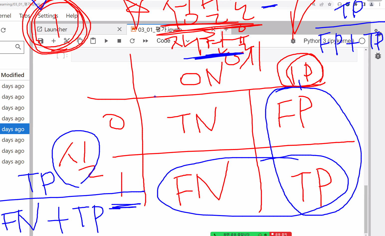
정확도 = 내가 맞춘 개수 / 전체 데이터 개수
균형이 안 맞은 이진 분류일 때는 정확도가 높게 나와 정확한 판단이 어렵다. 불균형한 이진분류일 때는 혼동행렬(정밀도, 재현율)을 가지고 판단한다.
y=0, y=1 실제값, 정답, 레이블
y^=0 y^=1 예측값
재현율 = 민감도 = TPR(true positive rate)
from sklearn.base import BaseEstimator
from sklearn.model_selection import train_test_split
import pandas as pd
from sklearn.metrics import accuracy_score
import numpy as np
class MyDummyClassifier(BaseEstimator): #클래스이름 옆에 ()하면 상속이다. BaseEstimator을 상속받겠다.
def fit(self, X, y=None):
pass
def predict(self, X):
pred = np.zeros((X.shape[0], 1)) #행은 데이터의 건수다. column = 레이블값 1
for i in range(X.shape[0]): #데이터 건수(행)을 가져다가
if X['Sex'].iloc[i] == 1: #성별이 1=남자라면
pred[i] = 0 #결과값에 0을 넣어줘라
else:
pred[i] = 1
return preddef fillna(df):
df['Age'].fillna(df['Age'].mean(),inplace=True)
df['Cabin'].fillna('N',inplace=True)
df['Embarked'].fillna('N',inplace=True)
df['Fare'].fillna(0, inplace=True)
return df
def drop_features(df):
df.drop(columns=['PassengerId', 'Name', 'Ticket'], inplace=True)
return df
def format_features(df):
from sklearn.preprocessing import LabelEncoder #함수안에 같이 넣어주는 것이 좋음
df['Cabin'] = df['Cabin'].str[:1] #Cabin의 첫 번째 글자만 추출
features=['Sex','Cabin','Embarked']
for feature in features:
le = LabelEncoder()
df[feature] = le.fit_transform(df[feature])
print(le.classes_) #레이블인코더 확인 할 때 = class
return df
def transform_features(df): #함수 3개 호출
df = fillna(df)
df = drop_features(df)
df = format_features(df)
return df
df = pd.read_csv('titanic.csv')
y = df['Survived']
X = df.drop(columns=['Survived'])
X = transform_features(X)
X_train,X_test,y_train,y_test = train_test_split(X,y,test_size=0.2,random_state=11)['female' 'male']
['A' 'B' 'C' 'D' 'E' 'F' 'G' 'N' 'T']
['C' 'N' 'Q' 'S']myclf = MyDummyClassifier()
myclf.fit(X_train,y_train)
pred = myclf.predict(X_test)
accuracy_score(y_test,pred)
0.8324022346368715from sklearn.metrics import confusion_matrixconfusion_matrix(y_test,pred)array([[103, 15],
[ 15, 46]], dtype=int64)#get_clf_eval = confusion,matrix,accuracy, precision, recall등의 평가를 한꺼번에 호출하는 함수
def get_clf_eval(y_test,pred):
from sklearn.metrics import accuracy_score,precision_score,recall_score,confusion_matrix
confusion = confusion_matrix(y_test,pred)
accuracy = accuracy_score(y_test,pred)
precision = precision_score(y_test,pred)
recall = recall_score(y_test,pred)
print('오차행렬')
print(confusion)
print(f'정확도:{accuracy:.4f}, 정밀도:{precision:.4f}, 재현율:{recall:.4f}')+머신러닝이나 sklearn 라이브러리에서 보이는 clf는 classifier(분류기)를 의미
- 교재 156p
{0} = index라 안 적어도 괜찮다. {.4f} = 소수 이하 4번째 자리까지
f'' = python3이후 버전부터 사용가능하다.
import pandas as pd
import numpy as np
from sklearn.model_selection import train_test_split # 데이터 나누닉
from sklearn.linear_model import LogisticRegression #이진분류라서 회귀모델 사용
df = pd.read_csv('titanic.csv')
y = df['Survived'] #df[] = 컬럼이름
x = df.drop(columns=['Survived']) #해당 컬럼만 제거하고 나머지 값들을 x로 가져온다. 원본에는 적용xdef fillna(df):
df['Age'].fillna(df['Age'].mean(),inplace=True)
df['Cabin'].fillna('N',inplace=True)
df['Embarked'].fillna('N',inplace=True)
df['Fare'].fillna(0, inplace=True)
return df
def drop_features(df):
df.drop(columns=['PassengerId', 'Name', 'Ticket'], inplace=True)
return df
def format_features(df):
from sklearn.preprocessing import LabelEncoder #함수안에 같이 넣어주는 것이 좋음
df['Cabin'] = df['Cabin'].str[:1] #Cabin의 첫 번째 글자만 추출
features=['Sex','Cabin','Embarked']
for feature in features:
le = LabelEncoder()
df[feature] = le.fit_transform(df[feature])
print(le.classes_) #레이블인코더 확인 할 때 = class
return df
def transform_features(df): #함수 3개 호출
df = fillna(df)
df = drop_features(df)
df = format_features(df)
return dfdf = pd.read_csv('titanic.csv')
y = df['Survived']
X = df.drop(columns=['Survived'])
X = transform_features(X)['female' 'male']
['A' 'B' 'C' 'D' 'E' 'F' 'G' 'N' 'T']
['C' 'N' 'Q' 'S']X_train,X_test,y_train,y_test = train_test_split(X,y,test_size=0.2,random_state=11)lr_clf = LogisticRegression(solver='liblinear') #모델만듦
lr_clf.fit(X_train,y_train)
pred = lr_clf.predict(X_test)
get_clf_eval(y_test,pred)+LogisticRegression 객체의 생성 인자로 입력되는 solver='liblinear'는 로지스틱 회귀의 최적화 알고리즘 유형을 지정하는 것이다. 보통 작은 데이터 세트의 이진 분류인 경우 solver는 liblinear가 약간 성능이 좋은 경향이 있다.
오차행렬
[[108  10]
 [ 14  47]]
정확도:0.8659, 정밀도:0.8246, 재현율:0.7705
정밀도/재현율 트레이드 오프
- 교재 157p
결정 임곗값(Threshold)을 조정해 정밀도나 재현율 수치를 높일 수 있다.
정밀도/재현율의 트레이드오프(Trade-off)는 정밀도와 재현율은 상호 보완적인 평가 지표이기 대문에 한 쪽을 강제로 높이면 다른 수치는 떨어지는 것을 정밀도/재현율 트레이드 오프(Trade-off)라고 한다.
pred #1= 생존, 0= 사망, 1차원array([1, 0, 0, 0, 0, 0, 0, 1, 0, 1, 0, 0, 0, 0, 0, 0, 0, 0, 0, 1, 0, 0,
0, 0, 0, 0, 0, 0, 0, 0, 1, 1, 0, 1, 0, 0, 0, 1, 0, 0, 0, 0, 1, 1,
1, 1, 1, 0, 1, 0, 0, 0, 0, 1, 0, 0, 0, 0, 0, 0, 0, 0, 0, 0, 0, 0,
1, 1, 1, 0, 0, 0, 0, 1, 0, 0, 0, 0, 1, 0, 1, 1, 1, 0, 1, 1, 0, 0,
1, 0, 0, 0, 0, 0, 1, 0, 1, 0, 0, 1, 1, 0, 1, 0, 1, 0, 0, 0, 0, 0,
0, 0, 0, 1, 0, 0, 0, 0, 1, 0, 0, 0, 0, 0, 0, 0, 0, 0, 1, 0, 1, 0,
1, 1, 1, 0, 1, 0, 0, 1, 1, 0, 0, 0, 0, 1, 0, 0, 1, 0, 0, 1, 1, 0,
1, 1, 0, 0, 1, 1, 0, 1, 0, 1, 0, 1, 1, 0, 0, 1, 0, 1, 0, 0, 0, 0,
0, 0, 1], dtype=int64)사이킷런의 분류 알고리즘은 예측 데이터가 특정 레이블(label, 결정 클래스 값)에 속하는 지를 계산하기 위해 먼저 개별 레이블별로 결정 확률을 구한다. 그리고 예측 확률이 큰 레이블 값으로 예측하게 된다.
#predict_proba()메서드 : 개별 데이터별로 예측 확률을 반환
pred_proba = lr_clf.predict_proba(X_test)#2차원, 1개의 데이터를 통해 2개의 결과값이 나옴- 0.44935225, 0.55064775 둘다 더하면 1이 됨
# 앞(0.44935225)이 될 것은 0이 될 확률, 뒤(0.55064775)에 것은 1이 될 확율np.concatenate([pred_proba,pred.reshape(-1,1)],axis=1) #(shift+tab) (a1, a2, ...) 튜플로 묶여 있음, The arrays must have the same shape = 같은 shape
#pred 1차원이라서 2차원을 바꿔주기 위해 reshape을 사용함 , axis=1 : 열단위로 붙여야 함array([[0.44935225, 0.55064775, 1. ],
[0.86335511, 0.13664489, 0. ],
[0.86429643, 0.13570357, 0. ],
[0.84968519, 0.15031481, 0. ],
[0.82343409, 0.17656591, 0. ],
[0.84231224, 0.15768776, 0. ],
[0.87095489, 0.12904511, 0. ],
[0.27228603, 0.72771397, 1. ],
[0.78185128, 0.21814872, 0. ],
[0.33185998, 0.66814002, 1. ],
[0.86178763, 0.13821237, 0. ],
[0.87058097, 0.12941903, 0. ],
[0.8642595 , 0.1357405 , 0. ],
[0.87065944, 0.12934056, 0. ],
[0.56033544, 0.43966456, 0. ],
[0.85003022, 0.14996978, 0. ],
[0.88954172, 0.11045828, 0. ],
[0.74250732, 0.25749268, 0. ],
[0.71120224, 0.28879776, 0. ],
[0.23776278, 0.76223722, 1. ],
[0.75684107, 0.24315893, 0. ],
[0.62428169, 0.37571831, 0. ],
[0.84655246, 0.15344754, 0. ],
[0.82711256, 0.17288744, 0. ],
[0.86825628, 0.13174372, 0. ],
[0.77003828, 0.22996172, 0. ],
[0.82946349, 0.17053651, 0. ],
[0.90336131, 0.09663869, 0. ],
[0.73372049, 0.26627951, 0. ],
[0.68847387, 0.31152613, 0. ],
[0.07646869, 0.92353131, 1. ],
[0.2253212 , 0.7746788 , 1. ],
[0.87161939, 0.12838061, 0. ],
[0.24075418, 0.75924582, 1. ],
[0.62711731, 0.37288269, 0. ],
[0.77003828, 0.22996172, 0. ],
[0.90554276, 0.09445724, 0. ],
[0.40602574, 0.59397426, 1. ],
[0.93043584, 0.06956416, 0. ],
[0.8765052 , 0.1234948 , 0. ],
[0.69797422, 0.30202578, 0. ],
[0.89664595, 0.10335405, 0. ],
[0.21993379, 0.78006621, 1. ],
[0.31565713, 0.68434287, 1. ],
[0.37942228, 0.62057772, 1. ],
[0.37932891, 0.62067109, 1. ],
[0.07161281, 0.92838719, 1. ],
[0.55777586, 0.44222414, 0. ],
[0.07914487, 0.92085513, 1. ],
[0.86803082, 0.13196918, 0. ],
[0.50790057, 0.49209943, 0. ],
[0.87065944, 0.12934056, 0. ],
[0.85576405, 0.14423595, 0. ],
[0.34870129, 0.65129871, 1. ],
[0.71558417, 0.28441583, 0. ],
[0.78853206, 0.21146794, 0. ],
[0.7461921 , 0.2538079 , 0. ],
[0.86429 , 0.13571 , 0. ],
[0.84079003, 0.15920997, 0. ],
[0.59838066, 0.40161934, 0. ],
[0.73532081, 0.26467919, 0. ],
[0.88705596, 0.11294404, 0. ],
[0.545528 , 0.454472 , 0. ],
[0.55326343, 0.44673657, 0. ],
[0.62583522, 0.37416478, 0. ],
[0.88363277, 0.11636723, 0. ],
[0.35181256, 0.64818744, 1. ],
[0.39903352, 0.60096648, 1. ],
[0.08300815, 0.91699185, 1. ],
[0.85072522, 0.14927478, 0. ],
[0.86778819, 0.13221181, 0. ],
[0.83070924, 0.16929076, 0. ],
[0.87649042, 0.12350958, 0. ],
[0.05959915, 0.94040085, 1. ],
[0.78735759, 0.21264241, 0. ],
[0.87065944, 0.12934056, 0. ],
[0.716541 , 0.283459 , 0. ],
[0.79159804, 0.20840196, 0. ],
[0.20303098, 0.79696902, 1. ],
[0.86429 , 0.13571 , 0. ],
[0.2400505 , 0.7599495 , 1. ],
[0.37123587, 0.62876413, 1. ],
[0.08369626, 0.91630374, 1. ],
[0.84018612, 0.15981388, 0. ],
[0.07766719, 0.92233281, 1. ],
[0.08973248, 0.91026752, 1. ],
[0.84723076, 0.15276924, 0. ],
[0.8624153 , 0.1375847 , 0. ],
[0.16539734, 0.83460266, 1. ],
[0.87065944, 0.12934056, 0. ],
[0.87065944, 0.12934056, 0. ],
[0.77003828, 0.22996172, 0. ],
[0.75416744, 0.24583256, 0. ],
[0.87065944, 0.12934056, 0. ],
[0.37932891, 0.62067109, 1. ],
[0.89883889, 0.10116111, 0. ],
[0.07361403, 0.92638597, 1. ],
[0.87897226, 0.12102774, 0. ],
[0.60197825, 0.39802175, 0. ],
[0.06738996, 0.93261004, 1. ],
[0.47948281, 0.52051719, 1. ],
[0.9046927 , 0.0953073 , 0. ],
[0.05673721, 0.94326279, 1. ],
[0.88180787, 0.11819213, 0. ],
[0.45587969, 0.54412031, 1. ],
[0.86133437, 0.13866563, 0. ],
[0.84974929, 0.15025071, 0. ],
[0.85072697, 0.14927303, 0. ],
[0.55502751, 0.44497249, 0. ],
[0.88426898, 0.11573102, 0. ],
[0.84747418, 0.15252582, 0. ],
[0.87269562, 0.12730438, 0. ],
[0.67538692, 0.32461308, 0. ],
[0.48275247, 0.51724753, 1. ],
[0.86825628, 0.13174372, 0. ],
[0.9159719 , 0.0840281 , 0. ],
[0.84194204, 0.15805796, 0. ],
[0.78872838, 0.21127162, 0. ],
[0.11141754, 0.88858246, 1. ],
[0.90534855, 0.09465145, 0. ],
[0.87071643, 0.12928357, 0. ],
[0.86905438, 0.13094562, 0. ],
[0.91525793, 0.08474207, 0. ],
[0.58196827, 0.41803173, 0. ],
[0.98025012, 0.01974988, 0. ],
[0.87071643, 0.12928357, 0. ],
[0.87219019, 0.12780981, 0. ],
[0.7119464 , 0.2880536 , 0. ],
[0.34348899, 0.65651101, 1. ],
[0.70226693, 0.29773307, 0. ],
[0.06738996, 0.93261004, 1. ],
[0.59805546, 0.40194454, 0. ],
[0.3288534 , 0.6711466 , 1. ],
[0.48644765, 0.51355235, 1. ],
[0.42864813, 0.57135187, 1. ],
[0.56346572, 0.43653428, 0. ],
[0.25853148, 0.74146852, 1. ],
[0.77643225, 0.22356775, 0. ],
[0.87632447, 0.12367553, 0. ],
[0.15009277, 0.84990723, 1. ],
[0.13434695, 0.86565305, 1. ],
[0.85072697, 0.14927303, 0. ],
[0.86772102, 0.13227898, 0. ],
[0.89628756, 0.10371244, 0. ],
[0.88613339, 0.11386661, 0. ],
[0.34797639, 0.65202361, 1. ],
[0.89917048, 0.10082952, 0. ],
[0.72997342, 0.27002658, 0. ],
[0.12221446, 0.87778554, 1. ],
[0.8171969 , 0.1828031 , 0. ],
[0.61865112, 0.38134888, 0. ],
[0.37370305, 0.62629695, 1. ],
[0.38348341, 0.61651659, 1. ],
[0.86463298, 0.13536702, 0. ],
[0.25161298, 0.74838702, 1. ],
[0.10388332, 0.89611668, 1. ],
[0.57648057, 0.42351943, 0. ],
[0.85476848, 0.14523152, 0. ],
[0.31415125, 0.68584875, 1. ],
[0.33907972, 0.66092028, 1. ],
[0.84347719, 0.15652281, 0. ],
[0.23261134, 0.76738866, 1. ],
[0.88859273, 0.11140727, 0. ],
[0.35220567, 0.64779433, 1. ],
[0.58554858, 0.41445142, 0. ],
[0.36143288, 0.63856712, 1. ],
[0.1363406 , 0.8636594 , 1. ],
[0.67797005, 0.32202995, 0. ],
[0.88600083, 0.11399917, 0. ],
[0.13946115, 0.86053885, 1. ],
[0.87095489, 0.12904511, 0. ],
[0.20616022, 0.79383978, 1. ],
[0.76719902, 0.23280098, 0. ],
[0.77437244, 0.22562756, 0. ],
[0.50324048, 0.49675952, 0. ],
[0.91079838, 0.08920162, 0. ],
[0.84970738, 0.15029262, 0. ],
[0.54874087, 0.45125913, 0. ],
[0.48192063, 0.51807937, 1. ]])threshold변수를 특정 값으로 설정하고 Binarizer 클래스를 객체로 생성한다. 생성된 Binarizer 객체의 fit_transform()메서드를 이용해 넘파이 ndarray를 입력하면 입력된 ndarry의 값을 지정된 threshold보다 같거나 작으면 0값으로, 크면 1값으로 변환해 반환한다.
from sklearn.preprocessing import Binarizer #전처리X=[[1,-1,2,],
[2,0,0],
[0,1.1,1.2]]
X[[1, -1, 2], [2, 0, 0], [0, 1.1, 1.2]]binarizer = Binarizer(threshold=1.1) #들어오는 데이터의 임계값을 설정, 기본값은 threshold=0.0 : 0까지는 0으로 나가고 0보다 크면 1로 나간다.binarizer.fit_transform(X) #fit에서는 정보를 모은다. #(threshold=1.1) : 1.1까지는 0으로 반환, 1.1보다 크면 1로 반환array([[0., 0., 1.],
[1., 0., 0.],
[0., 0., 1.]])- 교재 160P
LogisticRegression 객체의 predict_proba()메서드로 구한 각 클래스별 예측 확률값인 pred_proba 객체 변수에 분류 결정 임곗값(threshold)을 0.5로 지정한 Binarizer 클래스를 적용해 최종 예측값을 구함
custom_threshold=0.5pred_probaarray([[0.44935225, 0.55064775],
[0.86335511, 0.13664489],
[0.86429643, 0.13570357],
[0.84968519, 0.15031481],
[0.82343409, 0.17656591],
[0.84231224, 0.15768776],
[0.87095489, 0.12904511],
[0.27228603, 0.72771397],
[0.78185128, 0.21814872],
[0.33185998, 0.66814002],
[0.86178763, 0.13821237],
[0.87058097, 0.12941903],
[0.8642595 , 0.1357405 ],
[0.87065944, 0.12934056],
[0.56033544, 0.43966456],
[0.85003022, 0.14996978],
[0.88954172, 0.11045828],
[0.74250732, 0.25749268],
[0.71120224, 0.28879776],
[0.23776278, 0.76223722],
[0.75684107, 0.24315893],
[0.62428169, 0.37571831],
[0.84655246, 0.15344754],
[0.82711256, 0.17288744],
[0.86825628, 0.13174372],
[0.77003828, 0.22996172],
[0.82946349, 0.17053651],
[0.90336131, 0.09663869],
[0.73372049, 0.26627951],
[0.68847387, 0.31152613],
[0.07646869, 0.92353131],
[0.2253212 , 0.7746788 ],
[0.87161939, 0.12838061],
[0.24075418, 0.75924582],
[0.62711731, 0.37288269],
[0.77003828, 0.22996172],
[0.90554276, 0.09445724],
[0.40602574, 0.59397426],
[0.93043584, 0.06956416],
[0.8765052 , 0.1234948 ],
[0.69797422, 0.30202578],
[0.89664595, 0.10335405],
[0.21993379, 0.78006621],
[0.31565713, 0.68434287],
[0.37942228, 0.62057772],
[0.37932891, 0.62067109],
[0.07161281, 0.92838719],
[0.55777586, 0.44222414],
[0.07914487, 0.92085513],
[0.86803082, 0.13196918],
[0.50790057, 0.49209943],
[0.87065944, 0.12934056],
[0.85576405, 0.14423595],
[0.34870129, 0.65129871],
[0.71558417, 0.28441583],
[0.78853206, 0.21146794],
[0.7461921 , 0.2538079 ],
[0.86429 , 0.13571 ],
[0.84079003, 0.15920997],
[0.59838066, 0.40161934],
[0.73532081, 0.26467919],
[0.88705596, 0.11294404],
[0.545528 , 0.454472 ],
[0.55326343, 0.44673657],
[0.62583522, 0.37416478],
[0.88363277, 0.11636723],
[0.35181256, 0.64818744],
[0.39903352, 0.60096648],
[0.08300815, 0.91699185],
[0.85072522, 0.14927478],
[0.86778819, 0.13221181],
[0.83070924, 0.16929076],
[0.87649042, 0.12350958],
[0.05959915, 0.94040085],
[0.78735759, 0.21264241],
[0.87065944, 0.12934056],
[0.716541 , 0.283459 ],
[0.79159804, 0.20840196],
[0.20303098, 0.79696902],
[0.86429 , 0.13571 ],
[0.2400505 , 0.7599495 ],
[0.37123587, 0.62876413],
[0.08369626, 0.91630374],
[0.84018612, 0.15981388],
[0.07766719, 0.92233281],
[0.08973248, 0.91026752],
[0.84723076, 0.15276924],
[0.8624153 , 0.1375847 ],
[0.16539734, 0.83460266],
[0.87065944, 0.12934056],
[0.87065944, 0.12934056],
[0.77003828, 0.22996172],
[0.75416744, 0.24583256],
[0.87065944, 0.12934056],
[0.37932891, 0.62067109],
[0.89883889, 0.10116111],
[0.07361403, 0.92638597],
[0.87897226, 0.12102774],
[0.60197825, 0.39802175],
[0.06738996, 0.93261004],
[0.47948281, 0.52051719],
[0.9046927 , 0.0953073 ],
[0.05673721, 0.94326279],
[0.88180787, 0.11819213],
[0.45587969, 0.54412031],
[0.86133437, 0.13866563],
[0.84974929, 0.15025071],
[0.85072697, 0.14927303],
[0.55502751, 0.44497249],
[0.88426898, 0.11573102],
[0.84747418, 0.15252582],
[0.87269562, 0.12730438],
[0.67538692, 0.32461308],
[0.48275247, 0.51724753],
[0.86825628, 0.13174372],
[0.9159719 , 0.0840281 ],
[0.84194204, 0.15805796],
[0.78872838, 0.21127162],
[0.11141754, 0.88858246],
[0.90534855, 0.09465145],
[0.87071643, 0.12928357],
[0.86905438, 0.13094562],
[0.91525793, 0.08474207],
[0.58196827, 0.41803173],
[0.98025012, 0.01974988],
[0.87071643, 0.12928357],
[0.87219019, 0.12780981],
[0.7119464 , 0.2880536 ],
[0.34348899, 0.65651101],
[0.70226693, 0.29773307],
[0.06738996, 0.93261004],
[0.59805546, 0.40194454],
[0.3288534 , 0.6711466 ],
[0.48644765, 0.51355235],
[0.42864813, 0.57135187],
[0.56346572, 0.43653428],
[0.25853148, 0.74146852],
[0.77643225, 0.22356775],
[0.87632447, 0.12367553],
[0.15009277, 0.84990723],
[0.13434695, 0.86565305],
[0.85072697, 0.14927303],
[0.86772102, 0.13227898],
[0.89628756, 0.10371244],
[0.88613339, 0.11386661],
[0.34797639, 0.65202361],
[0.89917048, 0.10082952],
[0.72997342, 0.27002658],
[0.12221446, 0.87778554],
[0.8171969 , 0.1828031 ],
[0.61865112, 0.38134888],
[0.37370305, 0.62629695],
[0.38348341, 0.61651659],
[0.86463298, 0.13536702],
[0.25161298, 0.74838702],
[0.10388332, 0.89611668],
[0.57648057, 0.42351943],
[0.85476848, 0.14523152],
[0.31415125, 0.68584875],
[0.33907972, 0.66092028],
[0.84347719, 0.15652281],
[0.23261134, 0.76738866],
[0.88859273, 0.11140727],
[0.35220567, 0.64779433],
[0.58554858, 0.41445142],
[0.36143288, 0.63856712],
[0.1363406 , 0.8636594 ],
[0.67797005, 0.32202995],
[0.88600083, 0.11399917],
[0.13946115, 0.86053885],
[0.87095489, 0.12904511],
[0.20616022, 0.79383978],
[0.76719902, 0.23280098],
[0.77437244, 0.22562756],
[0.50324048, 0.49675952],
[0.91079838, 0.08920162],
[0.84970738, 0.15029262],
[0.54874087, 0.45125913],
[0.48192063, 0.51807937]])pred_proba[:,1]# : = 전부가져오기, 1 = 뒤에있는 것만 가져오기
#2차원으로 바꿔야 함, 한 행에 한 건 -> reshape(-1, 1)array([0.55064775, 0.13664489, 0.13570357, 0.15031481, 0.17656591,
0.15768776, 0.12904511, 0.72771397, 0.21814872, 0.66814002,
0.13821237, 0.12941903, 0.1357405 , 0.12934056, 0.43966456,
0.14996978, 0.11045828, 0.25749268, 0.28879776, 0.76223722,
0.24315893, 0.37571831, 0.15344754, 0.17288744, 0.13174372,
0.22996172, 0.17053651, 0.09663869, 0.26627951, 0.31152613,
0.92353131, 0.7746788 , 0.12838061, 0.75924582, 0.37288269,
0.22996172, 0.09445724, 0.59397426, 0.06956416, 0.1234948 ,
0.30202578, 0.10335405, 0.78006621, 0.68434287, 0.62057772,
0.62067109, 0.92838719, 0.44222414, 0.92085513, 0.13196918,
0.49209943, 0.12934056, 0.14423595, 0.65129871, 0.28441583,
0.21146794, 0.2538079 , 0.13571 , 0.15920997, 0.40161934,
0.26467919, 0.11294404, 0.454472 , 0.44673657, 0.37416478,
0.11636723, 0.64818744, 0.60096648, 0.91699185, 0.14927478,
0.13221181, 0.16929076, 0.12350958, 0.94040085, 0.21264241,
0.12934056, 0.283459 , 0.20840196, 0.79696902, 0.13571 ,
0.7599495 , 0.62876413, 0.91630374, 0.15981388, 0.92233281,
0.91026752, 0.15276924, 0.1375847 , 0.83460266, 0.12934056,
0.12934056, 0.22996172, 0.24583256, 0.12934056, 0.62067109,
0.10116111, 0.92638597, 0.12102774, 0.39802175, 0.93261004,
0.52051719, 0.0953073 , 0.94326279, 0.11819213, 0.54412031,
0.13866563, 0.15025071, 0.14927303, 0.44497249, 0.11573102,
0.15252582, 0.12730438, 0.32461308, 0.51724753, 0.13174372,
0.0840281 , 0.15805796, 0.21127162, 0.88858246, 0.09465145,
0.12928357, 0.13094562, 0.08474207, 0.41803173, 0.01974988,
0.12928357, 0.12780981, 0.2880536 , 0.65651101, 0.29773307,
0.93261004, 0.40194454, 0.6711466 , 0.51355235, 0.57135187,
0.43653428, 0.74146852, 0.22356775, 0.12367553, 0.84990723,
0.86565305, 0.14927303, 0.13227898, 0.10371244, 0.11386661,
0.65202361, 0.10082952, 0.27002658, 0.87778554, 0.1828031 ,
0.38134888, 0.62629695, 0.61651659, 0.13536702, 0.74838702,
0.89611668, 0.42351943, 0.14523152, 0.68584875, 0.66092028,
0.15652281, 0.76738866, 0.11140727, 0.64779433, 0.41445142,
0.63856712, 0.8636594 , 0.32202995, 0.11399917, 0.86053885,
0.12904511, 0.79383978, 0.23280098, 0.22562756, 0.49675952,
0.08920162, 0.15029262, 0.45125913, 0.51807937])pred_proba_1 = pred_proba[:,1].reshape(-1,1)
pred_proba_1array([[0.55064775],
[0.13664489],
[0.13570357],
[0.15031481],
[0.17656591],
[0.15768776],
[0.12904511],
[0.72771397],
[0.21814872],
[0.66814002],
[0.13821237],
[0.12941903],
[0.1357405 ],
[0.12934056],
[0.43966456],
[0.14996978],
[0.11045828],
[0.25749268],
[0.28879776],
[0.76223722],
[0.24315893],
[0.37571831],
[0.15344754],
[0.17288744],
[0.13174372],
[0.22996172],
[0.17053651],
[0.09663869],
[0.26627951],
[0.31152613],
[0.92353131],
[0.7746788 ],
[0.12838061],
[0.75924582],
[0.37288269],
[0.22996172],
[0.09445724],
[0.59397426],
[0.06956416],
[0.1234948 ],
[0.30202578],
[0.10335405],
[0.78006621],
[0.68434287],
[0.62057772],
[0.62067109],
[0.92838719],
[0.44222414],
[0.92085513],
[0.13196918],
[0.49209943],
[0.12934056],
[0.14423595],
[0.65129871],
[0.28441583],
[0.21146794],
[0.2538079 ],
[0.13571 ],
[0.15920997],
[0.40161934],
[0.26467919],
[0.11294404],
[0.454472 ],
[0.44673657],
[0.37416478],
[0.11636723],
[0.64818744],
[0.60096648],
[0.91699185],
[0.14927478],
[0.13221181],
[0.16929076],
[0.12350958],
[0.94040085],
[0.21264241],
[0.12934056],
[0.283459 ],
[0.20840196],
[0.79696902],
[0.13571 ],
[0.7599495 ],
[0.62876413],
[0.91630374],
[0.15981388],
[0.92233281],
[0.91026752],
[0.15276924],
[0.1375847 ],
[0.83460266],
[0.12934056],
[0.12934056],
[0.22996172],
[0.24583256],
[0.12934056],
[0.62067109],
[0.10116111],
[0.92638597],
[0.12102774],
[0.39802175],
[0.93261004],
[0.52051719],
[0.0953073 ],
[0.94326279],
[0.11819213],
[0.54412031],
[0.13866563],
[0.15025071],
[0.14927303],
[0.44497249],
[0.11573102],
[0.15252582],
[0.12730438],
[0.32461308],
[0.51724753],
[0.13174372],
[0.0840281 ],
[0.15805796],
[0.21127162],
[0.88858246],
[0.09465145],
[0.12928357],
[0.13094562],
[0.08474207],
[0.41803173],
[0.01974988],
[0.12928357],
[0.12780981],
[0.2880536 ],
[0.65651101],
[0.29773307],
[0.93261004],
[0.40194454],
[0.6711466 ],
[0.51355235],
[0.57135187],
[0.43653428],
[0.74146852],
[0.22356775],
[0.12367553],
[0.84990723],
[0.86565305],
[0.14927303],
[0.13227898],
[0.10371244],
[0.11386661],
[0.65202361],
[0.10082952],
[0.27002658],
[0.87778554],
[0.1828031 ],
[0.38134888],
[0.62629695],
[0.61651659],
[0.13536702],
[0.74838702],
[0.89611668],
[0.42351943],
[0.14523152],
[0.68584875],
[0.66092028],
[0.15652281],
[0.76738866],
[0.11140727],
[0.64779433],
[0.41445142],
[0.63856712],
[0.8636594 ],
[0.32202995],
[0.11399917],
[0.86053885],
[0.12904511],
[0.79383978],
[0.23280098],
[0.22562756],
[0.49675952],
[0.08920162],
[0.15029262],
[0.45125913],
[0.51807937]])custom_predict = Binarizer(threshold=custom_threshold).fit_transform(pred_proba_1)
#Binarizer(threshold=custom_threshold) = 임계값 0.5
#fit_transform(pred_proba_1) = 1일될 확률값# 오차행렬
# [[108 10]
# [ 14 47]]
# 정확도:0.8659, 정밀도:0.8246, 재현율:0.7705
get_clf_eval(y_test,custom_predict) #임계값 0.5 확인오차행렬
[[108 10]
[ 14 47]]
정확도:0.8659, 정밀도:0.8246, 재현율:0.7705custom_threshold = 0.4
custom_predict = Binarizer(threshold=custom_threshold).fit_transform(pred_proba_1)
get_clf_eval(y_test,custom_predict) #임계값 0.4 -> 정확도, 정밀도 떨어짐↓ 재현율은 올라감↑오차행렬
[[97 21]
[11 50]]
정확도:0.8212, 정밀도:0.7042, 재현율:0.8197custom_threshold = 0.6
custom_predict = Binarizer(threshold=custom_threshold).fit_transform(pred_proba_1)
get_clf_eval(y_test,custom_predict) #정확도, 정밀도 올라감↑ 재현율 내려감↓오차행렬
[[113 5]
[ 17 44]]
정확도:0.8771, 정밀도:0.8980, 재현율:0.7213thresholds = [0.4,0.45,0.5,0.55,0.6]
def get_eval_by_threshold(y_test,pred_proba_1,thresholds):
for custom_threshold in thresholds:
custom_predict = Binarizer(threshold=custom_threshold).fit_transform(pred_proba_1)
get_clf_eval(y_test,custom_predict)
get_eval_by_threshold(y_test,pred_proba_1,thresholds)오차행렬
[[97 21]
[11 50]]
정확도:0.8212, 정밀도:0.7042, 재현율:0.8197
오차행렬
[[105 13]
[ 13 48]]
정확도:0.8547, 정밀도:0.7869, 재현율:0.7869
오차행렬
[[108  10]
 [ 14  47]]
정확도:0.8659, 정밀도:0.8246, 재현율:0.7705
오차행렬
[[111 7]
[ 16 45]]
정확도:0.8715, 정밀도:0.8654, 재현율:0.7377
오차행렬
[[113 5]
[ 17 44]]
정확도:0.8771, 정밀도:0.8980, 재현율:0.7213- 교재 157p
output 잘못됨(임계치=0.5)
실습한 데이터가 맞음
[[108 10][ 14 47]]
정확도:0.8659, 정밀도:0.8246, 재현율:0.7705
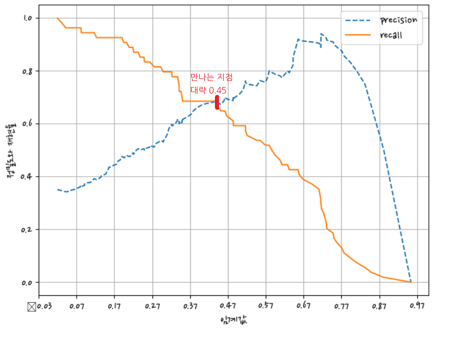
그래프에서 크로스되는 지점을 임계점으로 정한다.
precision_recall_curve()
임계값이 변하면 precision, recall값이 어떻게 변하는 지 보여줌
precision_recall_curve()의 인자로 실제 값 데이터 세트와 레이블 값이 1일 때의 예측 확률 값을 입력한다. 레이블 값이 1일 때의 예측 확률은 predict_proba(X_test)[:,1]로 predict_proba()의 반환 ndarray의 두 번째 칼럼(즉, 칼럼 인덱스 1)값에 해당하는 데이터 세트이다. precision_recall_curve()는 일반적으로 0.11~0.95 정도의 임곗값을 담은 넘파이 ndarray와 이 임곗값에 해당하는 정밀도 및 재현율 값을 담은 넘파이 ndarray를 반환한다.
from sklearn.metrics import precision_recall_curve#레이블 값이 1일 때의 예측 확률을 추출
precision_recall_curve(y_test,pred_proba_1) #y_true = y_test 결과값, probas_pred = 예측확률, pred_proba_1: 1에 대한 확률 값
#결과값 (array( : (로 시작된다는 것은 튜플이라는 뜻(array([0.37888199, 0.375 , 0.37735849, 0.37974684, 0.38216561,
0.37820513, 0.38064516, 0.38311688, 0.38562092, 0.38815789,
0.39072848, 0.39597315, 0.40136054, 0.41843972, 0.42142857,
0.42446043, 0.43065693, 0.43382353, 0.43703704, 0.44029851,
0.44360902, 0.4469697 , 0.44615385, 0.4496124 , 0.4453125 ,
0.44094488, 0.44444444, 0.44 , 0.44354839, 0.44715447,
0.45454545, 0.45833333, 0.46218487, 0.46610169, 0.47008547,
0.47413793, 0.47826087, 0.48245614, 0.48672566, 0.49107143,
0.4954955 , 0.5 , 0.50458716, 0.50925926, 0.51401869,
0.51886792, 0.52380952, 0.52884615, 0.53398058, 0.53921569,
0.54455446, 0.55 , 0.55555556, 0.56122449, 0.56701031,
0.57291667, 0.59139785, 0.59782609, 0.6043956 , 0.61111111,
0.61797753, 0.625 , 0.63218391, 0.63953488, 0.64705882,
0.64285714, 0.65060241, 0.65853659, 0.66666667, 0.675 ,
0.6835443 , 0.69230769, 0.68831169, 0.68421053, 0.68 ,
0.67567568, 0.68493151, 0.69444444, 0.70422535, 0.71428571,
0.71014493, 0.72058824, 0.73134328, 0.74242424, 0.75384615,
0.765625 , 0.76190476, 0.77419355, 0.78688525, 0.8 ,
0.79661017, 0.81034483, 0.8245614 , 0.83928571, 0.83636364,
0.83333333, 0.8490566 , 0.86538462, 0.8627451 , 0.88 ,
0.89795918, 0.89583333, 0.91489362, 0.93478261, 0.93181818,
0.93023256, 0.92857143, 0.95121951, 0.95 , 0.94871795,
0.94736842, 0.94594595, 0.94444444, 0.94285714, 0.94117647,
0.93939394, 0.9375 , 0.96774194, 0.96666667, 0.96551724,
0.96428571, 0.96296296, 0.96153846, 0.96 , 0.95833333,
0.95652174, 0.95454545, 0.95238095, 0.95 , 0.94736842,
0.94444444, 0.94117647, 0.9375 , 1. , 1. ,
1. , 1. , 1. , 1. , 1. ,
1. , 1. , 1. , 1. , 1. ,
1. , 1. , 1. ]),
array([1. , 0.98360656, 0.98360656, 0.98360656, 0.98360656,
0.96721311, 0.96721311, 0.96721311, 0.96721311, 0.96721311,
0.96721311, 0.96721311, 0.96721311, 0.96721311, 0.96721311,
0.96721311, 0.96721311, 0.96721311, 0.96721311, 0.96721311,
0.96721311, 0.96721311, 0.95081967, 0.95081967, 0.93442623,
0.91803279, 0.91803279, 0.90163934, 0.90163934, 0.90163934,
0.90163934, 0.90163934, 0.90163934, 0.90163934, 0.90163934,
0.90163934, 0.90163934, 0.90163934, 0.90163934, 0.90163934,
0.90163934, 0.90163934, 0.90163934, 0.90163934, 0.90163934,
0.90163934, 0.90163934, 0.90163934, 0.90163934, 0.90163934,
0.90163934, 0.90163934, 0.90163934, 0.90163934, 0.90163934,
0.90163934, 0.90163934, 0.90163934, 0.90163934, 0.90163934,
0.90163934, 0.90163934, 0.90163934, 0.90163934, 0.90163934,
0.8852459 , 0.8852459 , 0.8852459 , 0.8852459 , 0.8852459 ,
0.8852459 , 0.8852459 , 0.86885246, 0.85245902, 0.83606557,
0.81967213, 0.81967213, 0.81967213, 0.81967213, 0.81967213,
0.80327869, 0.80327869, 0.80327869, 0.80327869, 0.80327869,
0.80327869, 0.78688525, 0.78688525, 0.78688525, 0.78688525,
0.7704918 , 0.7704918 , 0.7704918 , 0.7704918 , 0.75409836,
0.73770492, 0.73770492, 0.73770492, 0.72131148, 0.72131148,
0.72131148, 0.70491803, 0.70491803, 0.70491803, 0.67213115,
0.6557377 , 0.63934426, 0.63934426, 0.62295082, 0.60655738,
0.59016393, 0.57377049, 0.55737705, 0.54098361, 0.52459016,
0.50819672, 0.49180328, 0.49180328, 0.47540984, 0.45901639,
0.44262295, 0.42622951, 0.40983607, 0.39344262, 0.37704918,
0.36065574, 0.3442623 , 0.32786885, 0.31147541, 0.29508197,
0.27868852, 0.26229508, 0.24590164, 0.24590164, 0.2295082 ,
0.21311475, 0.19672131, 0.18032787, 0.16393443, 0.14754098,
0.13114754, 0.1147541 , 0.09836066, 0.08196721, 0.06557377,
0.03278689, 0.01639344, 0. ]),
array([0.11573102, 0.11636723, 0.11819213, 0.12102774, 0.1234948 ,
0.12350958, 0.12367553, 0.12730438, 0.12780981, 0.12838061,
0.12904511, 0.12928357, 0.12934056, 0.12941903, 0.13094562,
0.13174372, 0.13196918, 0.13221181, 0.13227898, 0.13536702,
0.13570357, 0.13571 , 0.1357405 , 0.13664489, 0.1375847 ,
0.13821237, 0.13866563, 0.14423595, 0.14523152, 0.14927303,
0.14927478, 0.14996978, 0.15025071, 0.15029262, 0.15031481,
0.15252582, 0.15276924, 0.15344754, 0.15652281, 0.15768776,
0.15805796, 0.15920997, 0.15981388, 0.16929076, 0.17053651,
0.17288744, 0.17656591, 0.1828031 , 0.20840196, 0.21127162,
0.21146794, 0.21264241, 0.21814872, 0.22356775, 0.22562756,
0.22996172, 0.23280098, 0.24315893, 0.24583256, 0.2538079 ,
0.25749268, 0.26467919, 0.26627951, 0.27002658, 0.283459 ,
0.28441583, 0.2880536 , 0.28879776, 0.29773307, 0.30202578,
0.31152613, 0.32202995, 0.32461308, 0.37288269, 0.37416478,
0.37571831, 0.38134888, 0.39802175, 0.40161934, 0.40194454,
0.41445142, 0.41803173, 0.42351943, 0.43653428, 0.43966456,
0.44222414, 0.44497249, 0.44673657, 0.45125913, 0.454472 ,
0.49209943, 0.49675952, 0.51355235, 0.51724753, 0.51807937,
0.52051719, 0.54412031, 0.55064775, 0.57135187, 0.59397426,
0.60096648, 0.61651659, 0.62057772, 0.62067109, 0.62629695,
0.62876413, 0.63856712, 0.64779433, 0.64818744, 0.65129871,
0.65202361, 0.65651101, 0.66092028, 0.66814002, 0.6711466 ,
0.68434287, 0.68584875, 0.72771397, 0.74146852, 0.74838702,
0.75924582, 0.7599495 , 0.76223722, 0.76738866, 0.7746788 ,
0.78006621, 0.79383978, 0.79696902, 0.83460266, 0.84990723,
0.86053885, 0.8636594 , 0.86565305, 0.87778554, 0.88858246,
0.89611668, 0.91026752, 0.91630374, 0.91699185, 0.92085513,
0.92233281, 0.92353131, 0.92638597, 0.92838719, 0.93261004,
0.94040085, 0.94326279]))- precision_recall_curve()
Returns
precision(정밀도) : ndarray of shape (n_thresholds + 1,)
Precision values such that element i is the precision of
predictions with score >= thresholds[i] and the last element is 1.
recall(재현율) : ndarray of shape (n_thresholds + 1,)
Decreasing recall values such that element i is the recall of
predictions with score >= thresholds[i] and the last element is 0.
thresholds(임곗값) : ndarray of shape (n_thresholds,)
Increasing thresholds on the decision function used to compute
precision and recall. n_thresholds <= len(np.unique(probas_pred)).
임계값을 키우면 정밀도(precision)는 커진다. 그래서 결과값이 0 -> 1로 점점 커진다.
임계값이 낮으면 재현율(recall)이 커진다. 그래서 결과값이 1 -> 0으로 작아진다.
임계값(0.11573102)으로 시작한다.
#실제값 데이터 세트와 레이블 값이 1일 때의 예측 확률을 precision_recall_curve 인자로 입력
precisions, recalls, thresholds = precision_recall_curve(y_test,pred_proba_1)
#precision : ndarray of shape (n_thresholds + 1,)?
precisions.shape, recalls.shape, thresholds.shape ((148,), (148,), (147,))#반환된 임계값 배열 로우가 147건이므로 샘플로 10건만 추출하되, 임곗값을 15 step으로 추출
thr_index = np.arange(0,thresholds.shape[0], 15) #(0,thresholds.shape[0]) = 0~146 차례대로 값을 가져온다.
#(0,thresholds.shape[0], 15) = 15개씩 건너서 값을 가져온다
#15 = stepthr_index #위치값, 눈으로 확인하기 위해서 10개만 뽑음array([ 0, 15, 30, 45, 60, 75, 90, 105, 120, 135])thresholds[thr_index]#index위치의 임계값을 가져온다. np.round = 반올림array([0.11573102, 0.13174372, 0.14927478, 0.17288744, 0.25749268,
0.37571831, 0.49209943, 0.62876413, 0.75924582, 0.89611668])np.round(thresholds[thr_index],2) #index위치의 임계값을 가져온다. np.round = 반올림array([0.12, 0.13, 0.15, 0.17, 0.26, 0.38, 0.49, 0.63, 0.76, 0.9 ])np.round(precisions[thr_index],3)array([0.379, 0.424, 0.455, 0.519, 0.618, 0.676, 0.797, 0.93 , 0.964,
1. ])np.round(recalls[thr_index], 3)array([1. , 0.967, 0.902, 0.902, 0.902, 0.82 , 0.77 , 0.656, 0.443,
0.213])import matplotlib.pyplot as pltdef precision_recall_curve_plot(y_test,pred_proba_1):
from sklearn.metrics import precision_recall_curve
import matplotlib.pyplot as plt
precisions, recalls, thresholds = precision_recall_curve(y_test,pred_proba_1)
plt.figure(figsize=(8,6)) #틀의 비율 정해줌
threshold_boundary=thresholds.shape[0] #thresholds.shape[0]의 전체갯수(147)가 threshold_boundary가 들어감
plt.plot(thresholds, precisions[0:threshold_boundary],linestyle='--',label='precision') #x축에 임계값 , y축에 recall, precision
#thresholds(148개), precisions(147개) 둘의 갯수가 안 맞아서
#precisions[0:thresholds_boundary] 0~147 = 148개로 맞춰줌
plt.plot(thresholds, recalls[0:threshold_boundary],label='recall')
start,end = plt.xlim() #x축의 시작값, 끝나는 값 지정
plt.xticks(np.round(np.arange(start,end,0.1),2)) #arange=range #step을 0.1씩 눈금을 만들었다.
plt.xlabel('임계값') #x축제목
plt.ylabel('정밀도와 재현율') #y축제목
plt.legend() #범례
plt.grid() #눈금선
plt.show()precision_recall_curve_plot(y_test,pred_proba_1)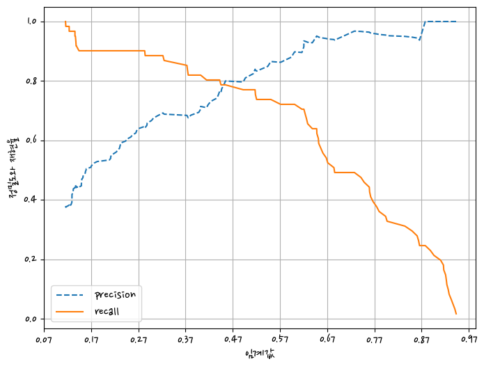
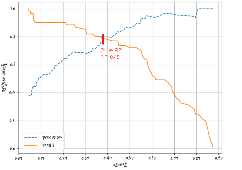
정밀도와 재현율가 밸런스가 맞는 지점 = 0.45
정밀도와 재현율의 맹점
- 교재 165p
정밀도와 재현율의 수치가 상호 보완할 수 있는 수준에서 적용돼어야 한다.
F1스코어
정밀도와 재현율을 결합한 지표이다.
정밀도와 재현율이 어느 한쪽으로 치우치지 않는 수치를 나타낼 때 상대적으로 높은 값을 가진다.
from sklearn.metrics import f1_scoref1_score(y_test,pred) # y_true : 정답,y_pred : 예측값 넣어주기0.7966101694915254def get_clf_eval(y_test,pred):
from sklearn.metrics import accuracy_score,precision_score,recall_score,confusion_matrix,f1_score
confusion = confusion_matrix(y_test,pred)
accuracy = accuracy_score(y_test,pred)
precision = precision_score(y_test,pred)
recall = recall_score(y_test,pred)
f1 = f1_score(y_test,pred)
print('오차행렬')
print(confusion)
print(f'정확도:{accuracy:.4f}, 정밀도:{precision:.4f}, 재현율:{recall:.4f}, F1:{f1:.4f}')
thresholds = [0.4,0.45,0.5,0.55,0.6]
def get_eval_by_threshold(y_test,pred_proba_1,thresholds):
for custom_threshold in thresholds:
custom_predict = Binarizer(threshold=custom_threshold).fit_transform(pred_proba_1)
print(f'임계값:{custom_threshold}')
get_clf_eval(y_test,custom_predict)
get_eval_by_threshold(y_test,pred_proba_1,thresholds)임계값:0.4
오차행렬
[[97 21]
 [11 50]]
정확도:0.8212, 정밀도:0.7042, 재현율:0.8197, F1:0.7576
임계값:0.45
오차행렬
[[105 13]
[ 13 48]]
정확도:0.8547, 정밀도:0.7869, 재현율:0.7869, F1:0.7869
임계값:0.5
오차행렬
[[108 10]
[ 14 47]]
정확도:0.8659, 정밀도:0.8246, 재현율:0.7705, F1:0.7966
임계값:0.55
오차행렬
[[111 7]
[ 16 45]]
정확도:0.8715, 정밀도:0.8654, 재현율:0.7377, F1:0.7965
임계값:0.6
오차행렬
[[113   5]
 [ 17  44]]
정확도:0.8771, 정밀도:0.8980, 재현율:0.7213, F1:0.8000쓰는 것은 사용하는 사람 마음이다.
본인이 어떻게 사용할 지 결정해야 한다.
ROC 곡선과 AUC
-교재 167P

ROC곡선의 아래쪽 면접의 값을 구한 값 = AUC
AUC는 1에 가까울수록 좋다.
재현율 = 민감도 = TPR
ROC곡선은 FPT이 변할 때 TPR(=recall)이 어떻게 변하는 지를 나타내는 곡선이다.
x축의 변화에 따른 y축의 변화
TNR= 특이성
TNR = TN / (FP+TN)
FPR = FP / (FP+FN) = 1 - TNR = 1 - 특이성
혼동행렬을 기반으로 한다.
-교재 169p
curve()는 그래프로 만들 수 있는 수치로 만들어 준다.
from sklearn.metrics import roc_curveroc_curve(y_test,pred_proba_1)(array([0. , 0. , 0. , 0. , 0. ,
0.00847458, 0.00847458, 0.01694915, 0.01694915, 0.02542373,
0.02542373, 0.02542373, 0.04237288, 0.04237288, 0.05932203,
0.05932203, 0.07627119, 0.07627119, 0.10169492, 0.10169492,
0.12711864, 0.12711864, 0.16949153, 0.16949153, 0.20338983,
0.20338983, 0.25423729, 0.25423729, 0.3220339 , 0.34745763,
0.55932203, 0.57627119, 0.59322034, 0.59322034, 0.60169492,
0.60169492, 0.61016949, 0.61864407, 0.66101695, 0.6779661 ,
0.69491525, 0.74576271, 0.77966102, 0.8220339 , 0.8220339 ,
0.84745763, 0.84745763, 1. ]),
array([0. , 0.01639344, 0.03278689, 0.06557377, 0.24590164,
0.24590164, 0.49180328, 0.49180328, 0.63934426, 0.63934426,
0.67213115, 0.70491803, 0.70491803, 0.72131148, 0.72131148,
0.73770492, 0.73770492, 0.7704918 , 0.7704918 , 0.78688525,
0.78688525, 0.80327869, 0.80327869, 0.81967213, 0.81967213,
0.8852459 , 0.8852459 , 0.90163934, 0.90163934, 0.90163934,
0.90163934, 0.90163934, 0.90163934, 0.91803279, 0.91803279,
0.95081967, 0.95081967, 0.96721311, 0.96721311, 0.96721311,
0.96721311, 0.96721311, 0.96721311, 0.96721311, 0.98360656,
0.98360656, 1. , 1. ]),
array([1.94326279, 0.94326279, 0.94040085, 0.93261004, 0.87778554,
0.86565305, 0.72771397, 0.68584875, 0.64779433, 0.63856712,
0.62629695, 0.62067109, 0.61651659, 0.60096648, 0.57135187,
0.55064775, 0.52051719, 0.51724753, 0.49209943, 0.454472 ,
0.44497249, 0.44222414, 0.41445142, 0.40194454, 0.37571831,
0.32202995, 0.28441583, 0.283459 , 0.23280098, 0.22996172,
0.14927478, 0.14927303, 0.14423595, 0.13866563, 0.13821237,
0.13664489, 0.1357405 , 0.13571 , 0.13196918, 0.13174372,
0.12941903, 0.12934056, 0.12904511, 0.12350958, 0.1234948 ,
0.11636723, 0.11573102, 0.01974988]))- roc_curve()
Returns
fpr : ndarray of shape (>2,) #x축
Increasing false positive rates such that element i is the false
positive rate of predictions with score >= thresholds[i].
tpr : ndarray of shape (>2,) #y축, 민감도
Increasing true positive rates such that element i is the true
positive rate of predictions with score >= thresholds[i].
thresholds : ndarray of shape = (n_thresholds,)
Decreasing thresholds on the decision function used to compute
fpr and tpr. thresholds[0] represents no instances being predicted
and is arbitrarily set to max(y_score) + 1.
def roc_curve_plot(y_test,pred_proba_1):
    from sklearn.metrics import roc_curve
    import matplotlib.pyplot as plt
    fprs, tprs, thresholds = roc_curve(y_test,pred_proba_1)
    plt.plot(fprs,tprs,label='ROC') #x축 = fprs, y축 = tprs
    plt.plot([0,1],[0,1], 'k--', label='Random') #x = [0,1],y = [0,1] , 50%되는 지점, 'k--' = 검은색 점선으로 표시해라
    plt.legend()
plt.show()roc_curve_plot(y_test,pred_proba_1)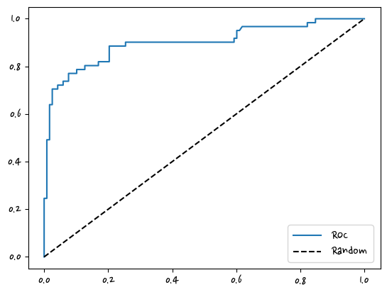
- 교재 171p
일반적으로 ROC 곡선은 FPR, TPR의 변화 값을 보는데 이용한다.
AUC 값은 ROC곡선 밑의 면적으로 구한 것으로서 일반적으로 1에 가까울수록 좋다.
보통의 경우 0.5이상의 AUC값을 가진다.
from sklearn.metrics import roc_auc_scoreroc_auc_score(y_test,pred_proba_1) #1인확률0.8986524034454015평가지표를 살펴봄. 이 모델이 쓸만 한지 평가지표
정확도만 가지고는 불균형한 이진분류에서 평가가 힘들어서
혼동행렬을 만들어서 정밀도, 재현율, f1스코드 등등 같이 본다
무조건 확인해야 하는 것이 아닌 상황에 따라서 확인한다.
def get_clf_eval(y_test,pred):
    from sklearn.metrics import accuracy_score,precision_score,recall_score,confusion_matrix,f1_score,roc_auc_score
    confusion = confusion_matrix(y_test,pred)
    accuracy = accuracy_score(y_test,pred)
    precision = precision_score(y_test,pred)
    recall = recall_score(y_test,pred)
    f1 = f1_score(y_test,pred)
    auc = roc_auc_score(y_test,pred_proba_1)
    print('오차행렬')
    print(confusion)
    print(f'정확도:{accuracy:.4f}, 정밀도:{precision:.4f}, 재현율:{recall:.4f}, F1:{f1:.4f}, AUC:{auc:.4f}')
-교재 172p
피마 인디언 당뇨병 예측
https://www.kaggle.com/datasets/uciml/pima-indians-diabetes-database
예측 변수(입력값)와 하나의 대상 변수(결과값, 레이블값)
당뇨병 원인으로 식습관과 유전을 꼽는다.
pima 인디원 데이터로 식습관의 영향을 살펴볼 수 있다.
import numpy as np
import pandas as pd
import matplotlib.pyplot as plt
from sklearn.model_selection import train_test_split
from sklearn.preprocessing import StandardScaler
from sklearn.linear_model import LogisticRegression
df = pd.read_csv('diabetes.csv') #DiabetesPedigreeFunction 유전(가중치), outcome(레이블값)
df.sample(3)| Pregnancies | Glucose | BloodPressure | SkinThickness | Insulin | BMI | DiabetesPedigreeFunction | Age | Outcome | |
|---|---|---|---|---|---|---|---|---|---|
| 732 | 2 | 174 | 88 | 37 | 120 | 44.5 | 0.646 | 24 | 1 |
| 738 | 2 | 99 | 60 | 17 | 160 | 36.6 | 0.453 | 21 | 0 |
| 260 | 3 | 191 | 68 | 15 | 130 | 30.9 | 0.299 | 34 | 0 |
df.info() #768 non-null = null값은 없다 , 모두 숫자형 -> 별도의 피처 인코딩 불필요<class 'pandas.core.frame.DataFrame'>
RangeIndex: 768 entries, 0 to 767
Data columns (total 9 columns):
# Column Non-Null Count Dtype
--- ------ -------------- -----
0 Pregnancies 768 non-null int64
1 Glucose 768 non-null int64
2 BloodPressure 768 non-null int64
3 SkinThickness 768 non-null int64
4 Insulin 768 non-null int64
5 BMI 768 non-null float64
6 DiabetesPedigreeFunction 768 non-null float64
7 Age 768 non-null int64
8 Outcome 768 non-null int64
dtypes: float64(2), int64(7)
memory usage: 54.1 KBdf.Outcome.value_counts() #유일값뽑고 몇 개씩있는지 0 500
1 268
Name: Outcome, dtype: int64X = df.drop(columns=['Outcome'])#outcom빼고 다 넣으면 된다. iloc, drop 써도 됨, 실제 데이터는 영향x
y = df.OutcomeX| Pregnancies | Glucose | BloodPressure | SkinThickness | Insulin | BMI | DiabetesPedigreeFunction | Age | |
|---|---|---|---|---|---|---|---|---|
| 0 | 6 | 148 | 72 | 35 | 0 | 33.6 | 0.627 | 50 |
| 1 | 1 | 85 | 66 | 29 | 0 | 26.6 | 0.351 | 31 |
| 2 | 8 | 183 | 64 | 0 | 0 | 23.3 | 0.672 | 32 |
| 3 | 1 | 89 | 66 | 23 | 94 | 28.1 | 0.167 | 21 |
| 4 | 0 | 137 | 40 | 35 | 168 | 43.1 | 2.288 | 33 |
| ... | ... | ... | ... | ... | ... | ... | ... | ... |
| 763 | 10 | 101 | 76 | 48 | 180 | 32.9 | 0.171 | 63 |
| 764 | 2 | 122 | 70 | 27 | 0 | 36.8 | 0.340 | 27 |
| 765 | 5 | 121 | 72 | 23 | 112 | 26.2 | 0.245 | 30 |
| 766 | 1 | 126 | 60 | 0 | 0 | 30.1 | 0.349 | 47 |
| 767 | 1 | 93 | 70 | 31 | 0 | 30.4 | 0.315 | 23 |
768 rows × 8 columns
y0 1
1 0
2 1
3 0
4 1
..
763 0
764 0
765 0
766 1
767 0
Name: Outcome, Length: 768, dtype: int64X_train,X_test,y_train,y_test = train_test_split(X,y,test_size=0.2,random_state=156,stratify=y)
lr_clf = LogisticRegression(solver='liblinear') #모델만듦
lr_clf.fit(X_train,y_train)
pred = lr_clf.predict(X_test)
pred_proba = lr_clf.predict_proba(X_test)[:,1]#stratify 교차검증할 때 비율따질 때
0    500
1    268
Name: Outcome, dtype: int64
비율이 불균형하다 -> 데이터를 나눌 때 비율이 불균형하면 성능이 좋지 않다.
-> 비율을 따져서 나눠야 한다. -> y값을 봐야 한다.
stratify=y 원래 데이터 비율에 맞춰서 데이터를 분류한다.
def get_clf_eval(y_test,pred,pred_proba_1): #(y_test,pred) 지역변수 pred = 결정값,pred_proba_1=확률값?
    from sklearn.metrics import accuracy_score,precision_score,recall_score,confusion_matrix,f1_score,roc_auc_score
    confusion = confusion_matrix(y_test,pred)
    accuracy = accuracy_score(y_test,pred)
    precision = precision_score(y_test,pred)
    recall = recall_score(y_test,pred)
    f1 = f1_score(y_test,pred)
    auc = roc_auc_score(y_test,pred_proba_1)
    print('오차행렬')
    print(confusion)
    print(f'정확도:{accuracy:.4f}, 정밀도:{precision:.4f}, 재현율:{recall:.4f}, F1:{f1:.4f}, AUC:{auc:.4f}')

def precision_recall_curve_plot(y_test,pred_proba_1):
    from sklearn.metrics import precision_recall_curve
    import matplotlib.pyplot as plt
    precisions, recalls, thresholds = precision_recall_curve(y_test,pred_proba_1)
    plt.figure(figsize=(8,6))
    threshold_boundary=thresholds.shape[0]
    plt.plot(thresholds, precisions[0:threshold_boundary],linestyle='--',label='precision')
    plt.plot(thresholds, recalls[0:threshold_boundary],label='recall')
    start,end = plt.xlim()
    plt.xticks(np.round(np.arange(start,end,0.1),2))
    plt.xlabel('임계값')
    plt.ylabel('정밀도와 재현율')
    plt.legend()
    plt.grid()
plt.show()get_clf_eval(y_test,pred,pred_proba)오차행렬
[[87 13]
[22 32]]
정확도:0.7727, 정밀도:0.7111, 재현율:0.5926, F1:0.6465, AUC:0.8083오차행렬
[[87 13][22 32]]
정확도:0.7727, 정밀도:0.7111, 재현율:0.5926, F1:0.6465, AUC:0.8083
정확도,정밀도는 높은데 재현율이 너무 낮다.
둘다 적절하게 높아야 f1스코어가 올라간다.
- 교재 175p
정밀도 재현율 곡선을 보고 임곗값별 정밀도와 재현율 값의 변화를 확인
precision_recall_curve_plot(y_test,pred_proba)C:\anaconda\lib\site-packages\IPython\core\pylabtools.py:151: UserWarning: Glyph 8722 (\N{MINUS SIGN}) missing from current font.
fig.canvas.print_figure(bytes_io, **kw)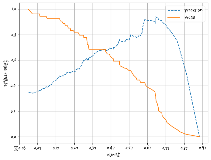
df.describe() #describe() 수치값 count, mean, std 등등 확인
#Glucose(포도당수치) 0이 될 수 없다.(잘못된 값)| Pregnancies | Glucose | BloodPressure | SkinThickness | Insulin | BMI | DiabetesPedigreeFunction | Age | Outcome | |
|---|---|---|---|---|---|---|---|---|---|
| count | 768.000000 | 768.000000 | 768.000000 | 768.000000 | 768.000000 | 768.000000 | 768.000000 | 768.000000 | 768.000000 |
| mean | 3.845052 | 120.894531 | 69.105469 | 20.536458 | 79.799479 | 31.992578 | 0.471876 | 33.240885 | 0.348958 |
| std | 3.369578 | 31.972618 | 19.355807 | 15.952218 | 115.244002 | 7.884160 | 0.331329 | 11.760232 | 0.476951 |
| min | 0.000000 | 0.000000 | 0.000000 | 0.000000 | 0.000000 | 0.000000 | 0.078000 | 21.000000 | 0.000000 |
| 25% | 1.000000 | 99.000000 | 62.000000 | 0.000000 | 0.000000 | 27.300000 | 0.243750 | 24.000000 | 0.000000 |
| 50% | 3.000000 | 117.000000 | 72.000000 | 23.000000 | 30.500000 | 32.000000 | 0.372500 | 29.000000 | 0.000000 |
| 75% | 6.000000 | 140.250000 | 80.000000 | 32.000000 | 127.250000 | 36.600000 | 0.626250 | 41.000000 | 1.000000 |
| max | 17.000000 | 199.000000 | 122.000000 | 99.000000 | 846.000000 | 67.100000 | 2.420000 | 81.000000 | 1.000000 |
- 교재 176p
잘못된 데이터 값 처리
히스토그램을 그려서 분포를 확인
plt.hist(df.Glucose,bins=100) #기본적으로 막대의 개수(bins)는 10이다.(array([ 5., 0., 0., 0., 0., 0., 0., 0., 0., 0., 0., 0., 0.,
0., 0., 0., 0., 0., 0., 0., 0., 0., 1., 0., 0., 0.,
0., 0., 3., 0., 1., 1., 1., 1., 3., 4., 4., 6., 4.,
7., 12., 9., 17., 10., 15., 20., 16., 20., 17., 20., 26., 22.,
19., 25., 25., 20., 18., 21., 18., 17., 17., 21., 25., 14., 25.,
12., 10., 10., 16., 13., 10., 11., 12., 16., 5., 9., 6., 11.,
5., 10., 4., 9., 7., 6., 5., 5., 7., 4., 3., 6., 10.,
4., 3., 5., 6., 2., 2., 5., 7., 2.]),
array([ 0. , 1.99, 3.98, 5.97, 7.96, 9.95, 11.94, 13.93,
15.92, 17.91, 19.9 , 21.89, 23.88, 25.87, 27.86, 29.85,
31.84, 33.83, 35.82, 37.81, 39.8 , 41.79, 43.78, 45.77,
47.76, 49.75, 51.74, 53.73, 55.72, 57.71, 59.7 , 61.69,
63.68, 65.67, 67.66, 69.65, 71.64, 73.63, 75.62, 77.61,
79.6 , 81.59, 83.58, 85.57, 87.56, 89.55, 91.54, 93.53,
95.52, 97.51, 99.5 , 101.49, 103.48, 105.47, 107.46, 109.45,
111.44, 113.43, 115.42, 117.41, 119.4 , 121.39, 123.38, 125.37,
127.36, 129.35, 131.34, 133.33, 135.32, 137.31, 139.3 , 141.29,
143.28, 145.27, 147.26, 149.25, 151.24, 153.23, 155.22, 157.21,
159.2 , 161.19, 163.18, 165.17, 167.16, 169.15, 171.14, 173.13,
175.12, 177.11, 179.1 , 181.09, 183.08, 185.07, 187.06, 189.05,
191.04, 193.03, 195.02, 197.01, 199. ]),
<BarContainer object of 100 artists>)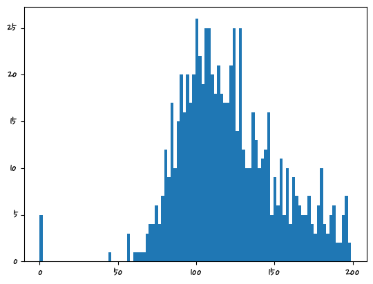
- 교재 177p
df.columnsIndex(['Pregnancies', 'Glucose', 'BloodPressure', 'SkinThickness', 'Insulin',
'BMI', 'DiabetesPedigreeFunction', 'Age', 'Outcome'],
dtype='object')zero_features = ['Glucose', 'BloodPressure', 'SkinThickness', 'Insulin','BMI']
total_count = df['Glucose'].count()
for feature in zero_features:
    zero_count = df[df[feature]==0][feature].count() #true인 것만 갯수를 셈
    print(f'{feature}컬럼의 0의 건수는 {zero_count}건 퍼센트는 {100*zero_count/total_count}%')
Glucose컬럼의 0의 건수는 5건 퍼센트는 0.6510416666666666%
BloodPressure컬럼의 0의 건수는 35건 퍼센트는 4.557291666666667%
SkinThickness컬럼의 0의 건수는 227건 퍼센트는 29.557291666666668%
Insulin컬럼의 0의 건수는 374건 퍼센트는 48.697916666666664%
BMI컬럼의 0의 건수는 11건 퍼센트는 1.4322916666666667%mean_zero_features = df[zero_features].mean() #zero_features의 평균df[zero_features] = df[zero_features].replace(0,mean_zero_features) #해당 컬럼값을 0을 평균값으로 대체한다.for feature in zero_features:
zero_count = df[df[feature]==0][feature].count() #true인 것만 갯수를 셈
print(f'{feature}컬럼의 0의 건수는 {zero_count}건 퍼센트는 {100*zero_count/total_count}%')Glucose컬럼의 0의 건수는 0건 퍼센트는 0.0%
BloodPressure컬럼의 0의 건수는 0건 퍼센트는 0.0%
SkinThickness컬럼의 0의 건수는 0건 퍼센트는 0.0%
Insulin컬럼의 0의 건수는 0건 퍼센트는 0.0%
BMI컬럼의 0의 건수는 0건 퍼센트는 0.0%minmax는 0~1사이 값으로 지정
standardscale 평균 0, 분산 1으로 바꿔준다. 가우시안 정규분포 비슷하게 바꿔준다.
하는 이유 : 데이터 값들이 범위가 제각각일 때 등등
X = df.drop(columns=['Outcome']) #모델만들고 학습
y = df.Outcome
scaler = StandardScaler()
X_scaled = scaler.fit_transform(X) #원본 놔두고 따른 곳에 저장
X_train,X_test,y_train,t_test = train_test_split(X_scaled,y,test_size=0.2,random_state=156,stratify=y)
lr_clf = LogisticRegression(solver='liblinear')
lr_clf.fit(X_train,y_train)
pred = lr_clf.predict(X_test)
pred_proba = lr_clf.predict_proba(X_test)[:,1]
get_clf_eval(y_test,pred,pred_proba)
# 오차행렬
# [[87 13]
#  [22 32]]
# 정확도:0.7727, 정밀도:0.7111, 재현율:0.5926, F1:0.6465, AUC:0.8083
오차행렬
[[90 10]
[21 33]]
정확도:0.7987, 정밀도:0.7674, 재현율:0.6111, F1:0.6804, AUC:0.8433thresholds = [0.3,0.33,0.36,0.39,0.42,0.45,0.48,0.5]
def get_eval_by_threshold(y_test,pred_proba_1,thresholds):
from sklearn.preprocessing import Binarizer
for custom_threshold in thresholds:
custom_predict = Binarizer(threshold=custom_threshold).fit_transform(pred_proba_1)
print(f'임계값:{custom_threshold}')
get_clf_eval(y_test,custom_predict,pred_proba_1) #인자값이 하나 늘어났다는 것이 무슨뜻? -> 3개가 들어가야 한다.
#y_test = 정답 ,custom_predict = Binarizer으로 조정한 값,pred_proba_1 = 확률값
get_eval_by_threshold(y_test,pred_proba.reshape(-1,1),thresholds)임계값:0.3
오차행렬
[[65 35]
[11 43]]
정확도:0.7013, 정밀도:0.5513, 재현율:0.7963, F1:0.6515, AUC:0.8433
임계값:0.33
오차행렬
[[71 29]
[11 43]]
정확도:0.7403, 정밀도:0.5972, 재현율:0.7963, F1:0.6825, AUC:0.8433
임계값:0.36
오차행렬
[[76 24]
[15 39]]
정확도:0.7468, 정밀도:0.6190, 재현율:0.7222, F1:0.6667, AUC:0.8433
임계값:0.39
오차행렬
[[78 22]
[16 38]]
정확도:0.7532, 정밀도:0.6333, 재현율:0.7037, F1:0.6667, AUC:0.8433
임계값:0.42
오차행렬
[[84 16]
[18 36]]
정확도:0.7792, 정밀도:0.6923, 재현율:0.6667, F1:0.6792, AUC:0.8433
임계값:0.45
오차행렬
[[85 15]
[18 36]]
정확도:0.7857, 정밀도:0.7059, 재현율:0.6667, F1:0.6857, AUC:0.8433
임계값:0.48
오차행렬
[[88 12]
[19 35]]
정확도:0.7987, 정밀도:0.7447, 재현율:0.6481, F1:0.6931, AUC:0.8433
임계값:0.5
오차행렬
[[90 10]
 [21 33]]
정확도:0.7987, 정밀도:0.7674, 재현율:0.6111, F1:0.6804, AUC:0.84332~3장에서 모델을 학습시켜서 사용, 전처리하는 과정, 모델학습시키고 평가를 배웠다.