지금까지 배운 것을 종합해서 타이타닉 데이터를 이용한 생존자 예측하기
변수 설명
- PassengerId : 각 승객의 고유 번호
- Survived : 생존 여부
0 = 사망
1 = 생존- Pclass : 객실 등급 - 승객의 사회적, 경제적 지위
1 = Upper
2 = Middle
3 = Lower- Name : 이름
- Sex : 성별
- Age : 나이
- SibSp : 동반한 Sibling(형제자매)와 Spouse(배우자)의 수
- Parch : 동반한 Parent(부모) Child(자식)의 수
- Ticket : 티켓의 고유넘버
- Fare : 티켓의 요금
- Cabin : 객실 번호
- Embarked : 승선한 항
C = Cherbourg
Q = Queenstown
S = Southampton
나머지 칼럼들을 이용해서 Survived 여부를 예측해보자!
EDA
import numpy as np
import pandas as pd
import matplotlib.pyplot as plt
import seaborn as sns
%matplotlib inline

titanic_df = pd.read_csv('./titanic_train.csv')
titanic_df.head(3)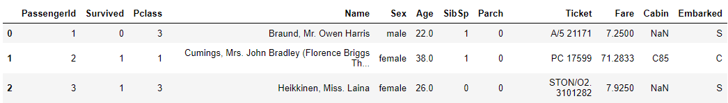
print(titanic_df.info())<class 'pandas.core.frame.DataFrame'>
RangeIndex: 891 entries, 0 to 890
Data columns (total 12 columns):
# Column Non-Null Count Dtype
--- ------ -------------- -----
0 PassengerId 891 non-null int64
1 Survived 891 non-null int64
2 Pclass 891 non-null int64
3 Name 891 non-null object
4 Sex 891 non-null object
5 Age 714 non-null float64
6 SibSp 891 non-null int64
7 Parch 891 non-null int64
8 Ticket 891 non-null object
9 Fare 891 non-null float64
10 Cabin 204 non-null object
11 Embarked 889 non-null object
dtypes: float64(2), int64(5), object(5)
memory usage: 83.7+ KB
NoneAge, Cabin, Embarked에 NULL 값이 존재한다.
Age는 평균값 대체하고, Cabin과 Embarked는 'N'이라는 새로운 값을 넣어주기로 한다.
titanic_df['Age'].fillna(titanic_df['Age'].mean(),inplace=True)
titanic_df['Cabin'].fillna('N',inplace=True) # 새로운 값
titanic_df['Embarked'].fillna('N',inplace=True) #새로운 값
print('피처별 Null 값 갯수\n',titanic_df.isnull().sum())
PassengerId, Name, Ticket는 생존자 예측이 불필요해 보이므로 제거한다.
titanic_df.drop(['PassengerId','Name','Ticket'],axis=1,inplace=True)Sex, Cabin, Embarked에 대해 분포를 확인한다.
print('Sex 값 분포 :\n',titanic_df['Sex'].value_counts())
print('\nCabin 값 분포 :\n',titanic_df['Cabin'].value_counts())
print('\nEmbarked 값 분포 :\n',titanic_df['Embarked'].value_counts())
Sex 값 분포 :
male 577
female 314
Name: Sex, dtype: int64
Cabin 값 분포 :
N 687
C23 C25 C27 4
G6 4
B96 B98 4
E101 3
...
B71 1
D48 1
E49 1
C99 1
C148 1
Name: Cabin, Length: 148, dtype: int64
Embarked 값 분포 :
S 644
C 168
Q 77
N 2Sex, Embarked는 괜찮아보이는데, Cabin은 unique값이 너무 많아보임
첫 글자만 떼서 변수를 다시 설정하자
titanic_df['Cabin'] = titanic_df['Cabin'].str[:1] # 첫 글자만 남기기
titanic_df['Cabin'].value_counts()
N 687
C 59
B 47
D 33
E 32
A 15
F 13
G 4
T 1
Name: Cabin, dtype: int64분포가 나름 괜찮아 보인다.
성별 사망자 수를 확인하고 시각화하기
# 성별 생존자 수
print(titanic_df.groupby(['Sex','Survived'])['Survived'].count())
# barplot -> 평균값을 보여줌
sns.barplot(x='Sex', y = 'Survived', data=titanic_df)
Sex Survived female 0 81 1 233 male 0 468 1 109 Name: Survived, dtype: int64
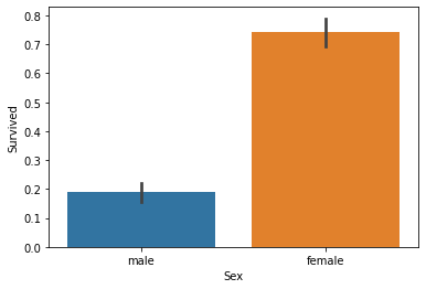
여성이 더 많이 생존한 것을 확인할 수 있다.
더 세분화해서 PClass(객실 등급)별 생존자 비율도 확인하자
sns.barplot(x='Pclass', y='Survived', hue='Sex', data=titanic_df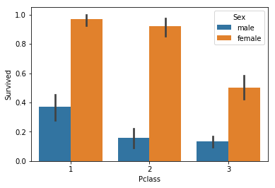
남/녀 모두 객실 등급이 높을수록 생존자가 많은 것을 볼 수 있다.
Encoding
문자열 값을 가지는 Cabin, Sex, Embarked에 대해 Label Encoding을 한다.
from sklearn.preprocessing import LabelEncoder

def encode_features(dataDF):
    features = ['Cabin', 'Sex', 'Embarked']
    for feature in features:
        le = LabelEncoder()
        le = le.fit(dataDF[feature])
        dataDF[feature] = le.transform(dataDF[feature])

    return dataDF

titanic_df = encode_features(titanic_df)
titanic_df.head()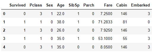
train/test 데이터 분리
X와 y를 데이터를 분리한 후 train/test 데이터세트를 분리한다.
train은 80%, test size는 20%로 분리 후 각 Shape을 확인한다.
y_titanic_df = titanic_df['Survived']
X_titanic_df= titanic_df.drop('Survived',axis=1)

from sklearn.model_selection import train_test_split
X_train, X_test, y_train, y_test=train_test_split(X_titanic_df, y_titanic_df, \
                                                  test_size=0.2, random_state=11)
print(X_train.shape, X_test.shape, y_train.shape,y_test.shape)
(712, 8) (179, 8) (712,) (179,)모델 적합 및 정확도 측정
DecisionTree, RandomForest, LogisticRegression 모델을 사용한다.
(X_train, y_train)을 각 모델에fit한 후, X_test에 대해predict한다.
from sklearn.tree import DecisionTreeClassifier
from sklearn.ensemble import RandomForestClassifier
from sklearn.linear_model import LogisticRegression
from sklearn.metrics import accuracy_score

# 결정트리, Random Forest, 로지스틱 회귀를 위한 사이킷런 Classifier 클래스 생성
dt_clf = DecisionTreeClassifier(random_state=11)
rf_clf = RandomForestClassifier(random_state=11)
# 사이킷런 버전 업으로 solver의 default 값이 변해서 고정시키기 위해 지정
lr_clf = LogisticRegression(solver='liblinear')

# DecisionTreeClassifier 학습/예측/평가
dt_clf.fit(X_train , y_train)
dt_pred = dt_clf.predict(X_test)
print('DecisionTreeClassifier 정확도: {0:.4f}'.format(accuracy_score(y_test, dt_pred)))

# RandomForestClassifier 학습/예측/평가
rf_clf.fit(X_train , y_train)
rf_pred = rf_clf.predict(X_test)
print('RandomForestClassifier 정확도:{0:.4f}'.format(accuracy_score(y_test, rf_pred)))

# LogisticRegression 학습/예측/평가
lr_clf.fit(X_train , y_train)
lr_pred = lr_clf.predict(X_test)
print('LogisticRegression 정확도: {0:.4f}'.format(accuracy_score(y_test, lr_pred)))
DecisionTreeClassifier 정확도: 0.7877
RandomForestClassifier 정확도:0.8547
LogisticRegression 정확도: 0.8659교차 검증과 GridSearchCV
머신러닝 과정은 위에서 다 끝났고, 번외로 test 데이터 나누기 전 타이타닉 데이터를 이용해서 교차 검증과 그리드 서치를 진행해본다.
교차검증
모델은 DecisionTree를 이용하고, cv=5로 진행한다.
from sklearn.model_selection import cross_val_score

scores = cross_val_score(dt_clf, X_titanic_df , y_titanic_df , cv=5)
for iter_count,accuracy in enumerate(scores):
    print("교차 검증 {0} 정확도: {1:.4f}".format(iter_count, accuracy))

print("평균 정확도: {0:.4f}".format(np.mean(scores)))
교차 검증 0 정확도: 0.7430
교차 검증 1 정확도: 0.7753
교차 검증 2 정확도: 0.7921
교차 검증 3 정확도: 0.7865
교차 검증 4 정확도: 0.8427
평균 정확도: 0.7879GridSearchCV
마찬가지로 모델은 DecisionTree를 이용하고, 파라미터는 이렇게 돌려본다.
- 'max_depth':[2,3,5,10]
- 'min_samples_split':[2,3,5]
- 'min_samples_leaf':[1,5,8]
from sklearn.model_selection import GridSearchCV

parameters = {'max_depth':[2,3,5,10],
             'min_samples_split':[2,3,5], 'min_samples_leaf':[1,5,8]}

# 4 * 3 * 3 * 5 번 학습
# refit은 기본값이 True
grid_dclf = GridSearchCV(dt_clf , param_grid=parameters , scoring='accuracy' , cv=5)
grid_dclf.fit(X_train , y_train)

print('GridSearchCV 최적 하이퍼 파라미터 :',grid_dclf.best_params_)
print('GridSearchCV 최고 정확도: {0:.4f}'.format(grid_dclf.best_score_))
best_dclf = grid_dclf.best_estimator_

# GridSearchCV의 최적 하이퍼 파라미터로 학습된 Estimator로 예측 및 평가 수행.
dpredictions = best_dclf.predict(X_test)
accuracy = accuracy_score(y_test , dpredictions)
print('테스트 세트에서의 DecisionTreeClassifier 정확도 : {0:.4f}'.format(accuracy))
GridSearchCV 최적 하이퍼 파라미터 : {'max_depth': 3, 'min_samples_leaf': 5, 'min_samples_split': 2}
GridSearchCV 최고 정확도: 0.7992
테스트 세트에서의 DecisionTreeClassifier 정확도 : 0.8715그리드 서치를 이용하니까 처음에 Descision Tree 모델 적합했을 때 보다 정확도가 많이 높아지는 것을 볼 수 있다!
강의 따라가면서 진행했는데 좀 정신이 없는 거 같아서 다음엔 Wine 데이터셋을 이용해서 처음부터 혼자 진행해보기로 함