PCA 실습 개요
scikit-learn은 sklearn.decomposition.PCA 클래스 제공
n_componets: PCA 축의 개수 (변환 차원)
PCA 이전에 입력 데이터의 개별 Feature에 대해 스케일링 필수!
PCA는 여러 Feature들의 값을 연산해야 하므로, Feature들의 스케일에 영향을 받음
일반적으로 평균이 0, 분산이 1인 표준 정규분포로 변환 (StandardScaler)
PCA 실습
다양한 데이터로 PCA 진행 후 모델 학습까지 해보자
iris 데이터 실습
데이터 로딩
from sklearn.datasets import load_iris
import pandas as pd
import matplotlib.pyplot as plt

iris = load_iris()

columns = ['sepal_length','sepal_width','petal_length','petal_width']
irisDF = pd.DataFrame(iris.data , columns=columns)
irisDF['target']=iris.target
irisDF.head(3)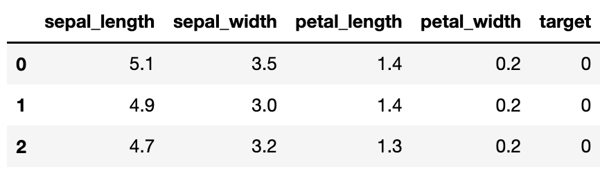
sepal_width와 sepal_length에 대해 각 품종별 산점도 나타내기
plt.scatter(irisDF[irisDF['target']==0]['sepal_length'],
            irisDF[irisDF['target']==0]['sepal_width'], marker='^',label='setosa')

plt.scatter(irisDF[irisDF['target']==1]['sepal_length'],
            irisDF[irisDF['target']==1]['sepal_width'], marker='s',label='versicolor')

plt.scatter(irisDF[irisDF['target']==2]['sepal_length'],
            irisDF[irisDF['target']==2]['sepal_width'], marker='o',label='virginica')

plt.legend()
plt.xlabel('sepal length')
plt.ylabel('sepal width')
plt.show()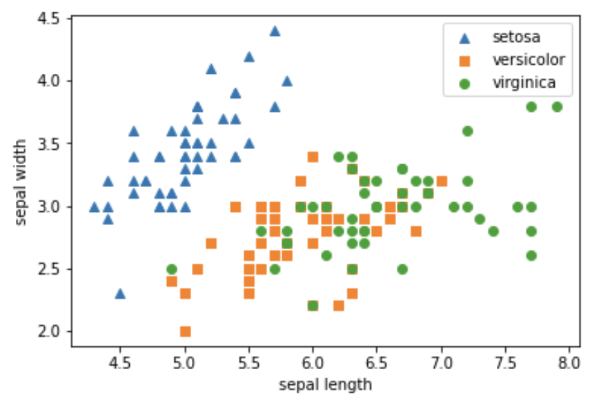
개별 Feature에 대해 Standard 스케일링 적용
from sklearn.preprocessing import StandardScaler

# Target 값을 제외한 모든 속성 값을 StandardScaler를 이용하여 표준 정규 분포를 가지는 값들로 변환
iris_scaled = StandardScaler().fit_transform(irisDF.iloc[:, :-1])
iris_scaled.shape
(150, 4)PCA 변환 수행
n_component = 2로 지정해서 Feature를 4개에서 2개로 줄임
from sklearn.decomposition import PCA

pca = PCA(n_components=2) # 2개의 주성분으로 압축

pca.fit(iris_scaled)
iris_pca = pca.transform(iris_scaled)
print(iris_pca.shape)
(150, 2)# PCA 변환된 데이터의 컬럼명을 각각 pca_component_1, pca_component_2로 명명
pca_columns=['pca_component_1','pca_component_2']
irisDF_pca = pd.DataFrame(iris_pca, columns=pca_columns)
irisDF_pca['target']=iris.target
irisDF_pca.head(3)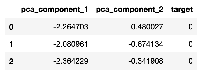
차원 축소된 두 개의 Feature로 각 품종별 산점도 시각화
plt.scatter(irisDF_pca[irisDF_pca['target']==0]['pca_component_1'],
            irisDF_pca[irisDF_pca['target']==0]['pca_component_2'], marker='^',label='setosa')

plt.scatter(irisDF_pca[irisDF_pca['target']==1]['pca_component_1'],
            irisDF_pca[irisDF_pca['target']==1]['pca_component_2'], marker='s',label='versicolor')

plt.scatter(irisDF_pca[irisDF_pca['target']==2]['pca_component_1'],
            irisDF_pca[irisDF_pca['target']==2]['pca_component_2'], marker='o',label='virginica')

plt.legend()
plt.xlabel('pca_component_1')
plt.ylabel('pca_component_2')
plt.show()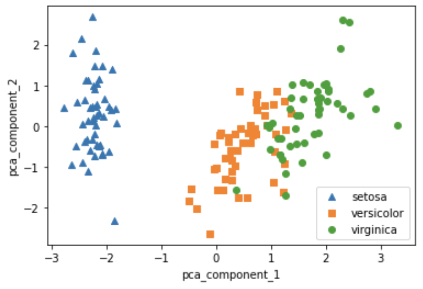
setosa는
pca_component_2로 잘 설명되는 것을 볼 수 있음
각 component의 변동성과 합계 확인하기
print(pca.explained_variance_ratio_)
print(np.sum(pca.explained_variance_ratio_))
[0.72962445 0.22850762]
0.9581320720000164두 개의 component만으로 약 95.8%를 설명하고 있음!
원본과 차원 축소 데이터의 예측 성능 비교
from sklearn.ensemble import RandomForestClassifier
from sklearn.model_selection import cross_val_score
import numpy as np

rcf = RandomForestClassifier(random_state=156)
scores = cross_val_score(rcf, iris.data, iris.target,scoring='accuracy',cv=3)
print('원본 데이터 교차 검증 개별 정확도:',scores)
print('원본 데이터 평균 정확도:', np.mean(scores))
원본 데이터 교차 검증 개별 정확도: [0.98 0.94 0.96]
원본 데이터 평균 정확도: 0.96pca_X = irisDF_pca[['pca_component_1', 'pca_component_2']]
scores_pca = cross_val_score(rcf, pca_X, iris.target, scoring='accuracy', cv=3 )
print('PCA 변환 데이터 교차 검증 개별 정확도:',scores_pca)
print('PCA 변환 데이터 평균 정확도:', np.mean(scores_pca))PCA 변환 데이터 교차 검증 개별 정확도: [0.88 0.88 0.88]
PCA 변환 데이터 평균 정확도: 0.88약간 차이가 나긴 하지만, 준수한 성능을 보여주고 있음
만약 개별 Feature들이 서로 상관관계가 높은 것들이 많이 있는 데이터의 경우 PCA를 진행해도 성능에 큰 변화가 생기지 않음!
신용카드 데이터 실습
데이터 출처: https://archive.ics.uci.edu/ml/datasets/default+of+credit+card+clients
데이터 로드
엑셀 파일 열어서 필요 없는 부분 파악하고 적절히 전처리 진행 (헤더, ID 칼럼 등)
# header로 의미없는 첫행 제거, iloc로 기존 id 제거
import pandas as pd
pd.set_option('display.max_columns', 30)

df = pd.read_excel('pca_credit_card.xls', header=1, sheet_name='Data').iloc[:,1:]
print(df.shape)
df.head(3)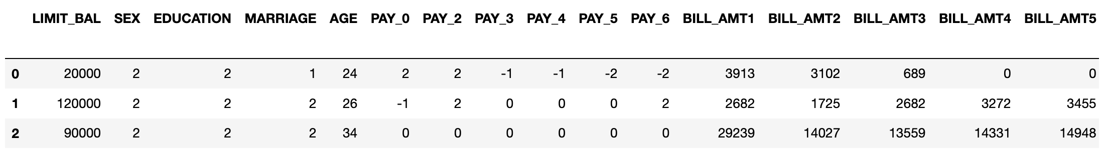
위에 표가 뒤에 좀 잘렸는데, 서로 비슷한 칼럼들이 좀 있음
Feature 이름 적절히 변경 후 Feature와 Target 데이터 분리
df.rename(columns={'PAY_0':'PAY_1','default payment next month':'default'}, inplace=True)
y_target = df['default']
X_features = df.drop('default', axis=1)X_features.info()<class 'pandas.core.frame.DataFrame'>
RangeIndex: 30000 entries, 0 to 29999
Data columns (total 23 columns):
# Column Non-Null Count Dtype
--- ------ -------------- -----
0 LIMIT_BAL 30000 non-null int64
1 SEX 30000 non-null int64
2 EDUCATION 30000 non-null int64
3 MARRIAGE 30000 non-null int64
4 AGE 30000 non-null int64
5 PAY_1 30000 non-null int64
6 PAY_2 30000 non-null int64
7 PAY_3 30000 non-null int64
8 PAY_4 30000 non-null int64
9 PAY_5 30000 non-null int64
10 PAY_6 30000 non-null int64
11 BILL_AMT1 30000 non-null int64
12 BILL_AMT2 30000 non-null int64
13 BILL_AMT3 30000 non-null int64
14 BILL_AMT4 30000 non-null int64
15 BILL_AMT5 30000 non-null int64
16 BILL_AMT6 30000 non-null int64
17 PAY_AMT1 30000 non-null int64
18 PAY_AMT2 30000 non-null int64
19 PAY_AMT3 30000 non-null int64
20 PAY_AMT4 30000 non-null int64
21 PAY_AMT5 30000 non-null int64
22 PAY_AMT6 30000 non-null int64
dtypes: int64(23)
memory usage: 5.3 MB히트맵으로 Feature별 상관관계를 파악해보자
import seaborn as sns
import matplotlib.pyplot as plt

corr = X_features.corr()
plt.figure(figsize=(14,14))

sns.heatmap(corr, annot=True, fmt='.1g')
plt.show()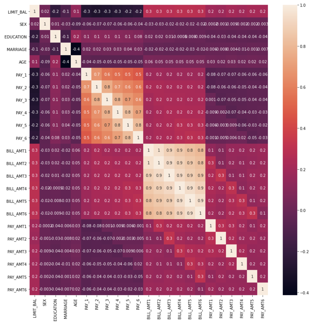
BILL_AMT Feature간에 상관관계가 매우 높게 나온다.
이를 대상으로 PCA로 차원 축소를 진행하자
from sklearn.decomposition import PCA
from sklearn.preprocessing import StandardScaler

# BILL_AMT1 ~ BILL_AMT6까지 6개의 속성명 생성
cols_bill = ['BILL_AMT'+str(i) for i in range(1, 7)]
print('대상 속성명:', cols_bill)

# 2개의 PCA 속성을 가진 PCA 객체 생성하고, explained_variance_ratio_ 계산을 위해 fit( ) 호출
scaler = StandardScaler()
df_cols_scaled = scaler.fit_transform(X_features[cols_bill])

pca = PCA(n_components=2)
pca.fit(df_cols_scaled)
print('PCA Component별 변동성:', pca.explained_variance_ratio_)
대상 속성명: ['BILL_AMT1', 'BILL_AMT2', 'BILL_AMT3', 'BILL_AMT4', 'BILL_AMT5', 'BILL_AMT6']
PCA Component별 변동성: [0.90555253 0.0509867 ]2개의 component로 6개의 Feature의 약 95.5%를 설명한다.
이제 원본 데이터와 전체 데이터에 대해 PCA를 진행한 것의 성능을 비교해보자
원본 데이터의 성능은 다음과 같다.
import numpy as np
from sklearn.ensemble import RandomForestClassifier
from sklearn.model_selection import cross_val_score

rcf = RandomForestClassifier(n_estimators=300, random_state=156)
scores = cross_val_score(rcf, X_features, y_target, scoring='accuracy', cv=3 )

print('CV=3 인 경우의 개별 Fold세트별 정확도:',scores)
print('평균 정확도:{0:.4f}'.format(np.mean(scores)))
CV=3 인 경우의 개별 Fold세트별 정확도: [0.8083 0.8196 0.8232]
평균 정확도:0.8170전체 데이터에 대해 6개의 component로 PCA한 것의 성능은 다음과 같다.
from sklearn.decomposition import PCA
from sklearn.preprocessing import StandardScaler

# 원본 데이터셋에 먼저 StandardScaler적용
scaler = StandardScaler()
df_scaled = scaler.fit_transform(X_features)

# 6개의 Component를 가진 PCA 변환을 수행하고 cross_val_score( )로 분류 예측 수행.
pca = PCA(n_components=6)
df_pca = pca.fit_transform(df_scaled)
scores_pca = cross_val_score(rcf, df_pca, y_target, scoring='accuracy', cv=3)

print('CV=3 인 경우의 PCA 변환된 개별 Fold세트별 정확도:',scores_pca)
print('PCA 변환 데이터 셋 평균 정확도:{0:.4f}'.format(np.mean(scores_pca)))
Feature의 갯수를 대폭 줄였는데, 성능에 큰 차이가 없다!