[ML] 차원 축소 - LDA (Linear Discriminant Analysis)

LDA 개요

LDA, Linear Discriminant Analysis, 선형 판별 분석

PCA와 매우 유사함

• PCA처럼 입력 데이터 세트를 저차원 공간에 투영해 차원을 축소하는 기법

• 중요한 차이는 LDA는 지도학습의 분류에서 사용하기 쉽도록 개별 클래스를 분별할 수 있는 기준을 최대한 유지하면서 차원 축소

• PCA는 입력 데이터의 변동성의 가장 큰 축을 찾았지만, LDA는 입력 데이터의 결정값 클래스를 최대한 분리할 수 있는 축을 찾음

• LDA는 같은 클래스의 데이터는 최대한 근접해서, 다른 클래스의 데이터는 최대한 떨어뜨리는 축 매핑 진행

LDA 차원 축소 방식
특정 공간상에서 클래스 분리를 최대화하는 축을 찾기 위해 클래스 간 분산과 클래스 내부 분산의 비율을 최대화하는 방식으로 축소
-> 클래스 간 분산은 최대한 크게, 클래스 내 분산은 최대한 작게

LDA 절차

1. 클래스 내부와 클래스 간 분산 행렬을 구하고, 이 두 개의 행렬은 입력 데이터의 결정 값 클래스별로 개별 Feature의 평균 벡터를 기반으로 구함

2. 클래스 내부 분산 행렬을 $S_W$, 클래스 간 분상 행렬을 $S_B$라고 하면, 다음 식으로 두 행렬을 고유벡터로 분해할 수 있음

3. 고윳값이 가장 큰 순으로 K개(LDA변환 차수만큼) 추출

4. 고윳값이 가장 큰 순으로 추출된 고유벡터를 이용해 새롭게 입력 데이터를 변환

LDA 실습

scikit-learn은 sklearn.discriminant_anlysis.LinearDiscriminantAnalysis 클래스 제공

LDA도 스케일링이 선수되어야 함
전체 코드는 PCA와 거의 유사한데, fit()할 때, Target 값이 들어와야 함
-> 그래서 사실 LDA는 비지도학습이 아님

from sklearn.discriminant_analysis import LinearDiscriminantAnalysis
from sklearn.preprocessing import StandardScaler
from sklearn.datasets import load_iris

iris = load_iris()
iris_scaled = StandardScaler().fit_transform(iris.data)

lda = LinearDiscriminantAnalysis(n_components=2)
# fit()호출 시 target값 입력 
lda.fit(iris_scaled, iris.target)
iris_lda = lda.transform(iris_scaled)
print(iris_lda.shape)

(150, 2)

import pandas as pd
import matplotlib.pyplot as plt

lda_columns=['lda_component_1','lda_component_2']
irisDF_lda = pd.DataFrame(iris_lda,columns=lda_columns)
irisDF_lda['target']=iris.target

#setosa는 세모, versicolor는 네모, virginica는 동그라미로 표현
markers=['^', 's', 'o']

#setosa의 target 값은 0, versicolor는 1, virginica는 2. 각 target 별로 다른 shape으로 scatter plot
for i, marker in enumerate(markers):
    x_axis_data = irisDF_lda[irisDF_lda['target']==i]['lda_component_1']
    y_axis_data = irisDF_lda[irisDF_lda['target']==i]['lda_component_2']

    plt.scatter(x_axis_data, y_axis_data, marker=marker,label=iris.target_names[i])

plt.legend(loc='upper right')
plt.xlabel('lda_component_1')
plt.ylabel('lda_component_2')
plt.show()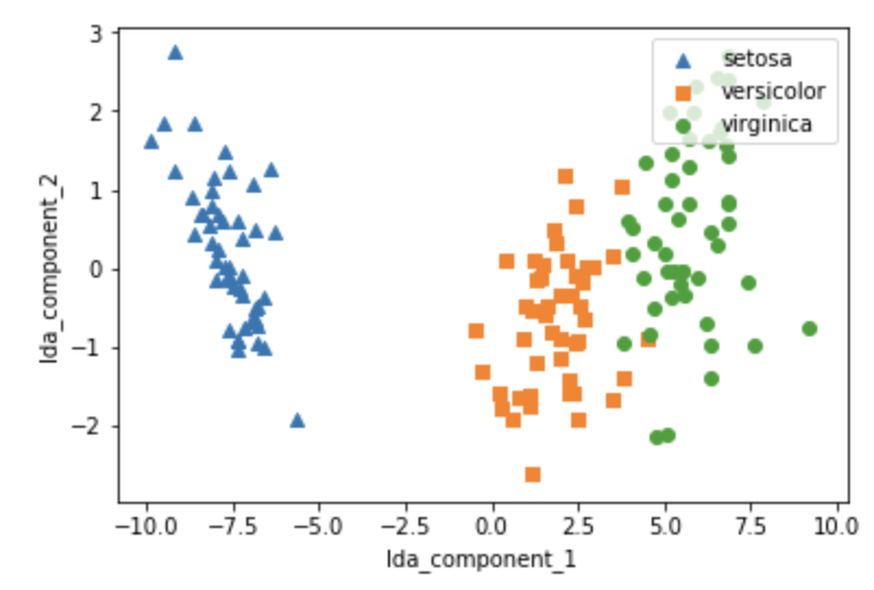

세 집단이 거의 겹치지 않고 잘 분류 된다!
앞에서 한 PCA 그림과 비교해보기