
기본 컨셉 코드
import numpy as np
from numpy.ma import array, masked_array, masked_values, masked_outside

vec1 = np.round(np.linspace(0.1,1,5), 3)
print('vec1: ', vec1)
print('array: ', array(vec1, mask = [0,0,0,1,0]))
# print(type(array(vec1, mask = [0,0,0,1,0])))
print('masked_array: ', masked_array(vec1, mask = [0,0,0,1,0]))
# print(type(masked_array(vec1, mask = [0,0,0,1,0])))
print('masked_outside: ', masked_outside(vec1,0.2,0.9), '\n')

vec2 = [0,1,2,3,4,-9999]
print('vec2: ', vec2)
print('masked_values: ', masked_values(vec2,-9999))
print('masked_values & filled: ', masked_values(vec2,-9999).filled(5555))
vec1: [0.1 0.325 0.55 0.775 1. ]
array: [0.1 0.325 0.55 -- 1.0]
masked_array: [0.1 0.325 0.55 -- 1.0]
masked_outside: [-- 0.325 0.55 0.775 --]
vec2: [0, 1, 2, 3, 4, -9999]
masked_values: [0 1 2 3 4 --]
masked_values & filled: [ 0 1 2 3 4 5555]⭐️ Pruning은 사용하지 않는 weight에 대하여 mask를 씌워 계산하게 된다.
이러한 mask테크닉은 NLP모델인 transformer에서도 decoder부분을 학습 시킬 때 현재의 단어 이후의 단어들의 영향을 받지 않데 할 때 쓰이는 등 다양한 용도로 사용할 수 있다.
Pruning이란
✔️ Pruning을 통해 얻는 것
- Inference speed
- Regularization (lessen model complexity) brings generalization
✔️ Pruning을 통해 잃는 것
- Information loss
- The granularity(세분성 - 얽히게 자르느냐 안 얽히게 자르느냐) affects the efficiency of hardware accelerator design
참고 자료
https://medium.com/@souvik.paul01/pruning-in-deep-learning-models-1067a19acd89
✔️ Pruning과 Dropout 차이
Pruning은 한번 잘라낸 가지를 다시 복원하지 않지만 Dropout은 weight의 사용을 껏다 켰다를 반복한다.
✔️ Pruning, Fine-Tuning psudo algorithm
https://arxiv.org/pdf/2003.03033.pdf -> Figure1
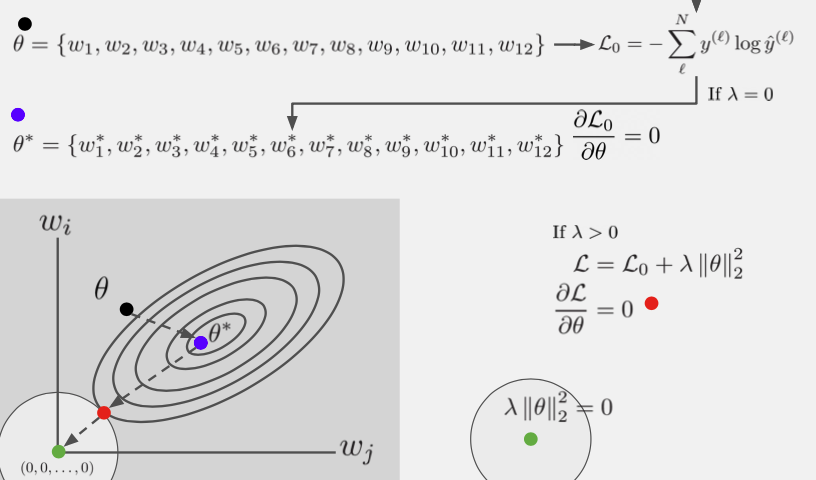
✔️ Regularization관점
Regularization은 overfitting을 막기 위한 term을 추가 해 준 작업인데 이 term은 파라미터 크기에 dependent하기 때문에 pruning행위는 Regularization term에 직접적인 영향을 미치게 된다.
출처 : Naver BoostCamp AI Tech - edwith 강의
여러 Pruning들
전반적인 내용은 해당 링크 참고
https://towardsdatascience.com/the-lottery-ticket-hypothesis-a-survey-d1f0f62f8884
✔️ Pruning방법은 정말 다양한 방법이 존재하고 이런 방법을 결정짓는 다양한 기준들이 존재한다.
✔️ Structed Pruning VS Unstructed Pruning
- Structed Pruning : 커다랗게 규격을 잡아 기준에 맞게 pruning을 진행하고 규격단위로 잘라내기 때문에 hardware단위로 optimize잘된다. => pruning진행 후 weight가 0인 것들도 좀 남게 된다.
- Unstructed Pruning : 구조화 하지 않고 잘라내기에 얽힌 모양이 나오게 된다.=> pruning진행 후 weight가 0인 것들이 중점적으로 제거된다.
✔️ Iterative pruning
http://proceedings.mlr.press/v119/tan20a/tan20a.pdf -> Algorithm1참고
Lottery ticket hypothesis
참고 자료
https://medium.com/analytics-vidhya/rigging-the-lottery-training-method-of-high-speed-and-high-precision-sparse-networks-without-2340b0461d55
https://arxiv.org/pdf/1803.03635.pdf
아래의 내용은 참고 자료의 부가 설명이다.
✔️ 핵심 가정은 원래 네트워크와 비슷한 성능을 내는 가지를 쳐낸 네트워크가 존재 할 것이라고 가정
💡 일단 original network을 알아야 lottery ticket을 알 수 있다.(original에 사용된 initialize값들을 사용하지 않게 되면 lottery ticket효과가 사라진다고 한다.)
💡 lottery ticket의 존재성은 밝혔으나 얻어내기 위해서는 많은 비용이 필요
✔️ Iterative Magnitude Pruning
initialized값 설정 후 train 시킨 다음 prune하는 과정을 반복
✔️ Iterative Magnitude Pruning with Rewinding
initialize값 설정 후 train 시킨 다음 prune하는 과정을 반복하는데 이 중 iteration을 돌다가 k번째에서의 weight를 저장 한 다음 이 값을 initialize값으로 사용
이때, k번째 weight에 noise를 넣어 수행을 해 주는데 이는 noise를 넣지 않게 되면 계속 동일한 initialize값을 사용하게 됨으로 의미가 사라지기 때문이다.
Pruning code
✔️ 처음 model을 prune하게 되면 오히려 model size가 커지는 현상을 볼 수 있는데 이는 mask가 추가되어 초기에 크기가 커져 보이는 것이고 이 마스크를 적용하면 원본과 모델은 동일한 사이즈이나 정확도는 다소 낮지만 속도가 빠른 것을 확인할 수 있다.
module = model.conv1

device = 'cpu'
test(model=model, device=device, test_loader=test_loader)
LeNet(
(conv1): Conv2d(1, 6, kernel_size=(3, 3), stride=(1, 1))
(conv2): Conv2d(6, 16, kernel_size=(3, 3), stride=(1, 1))
(fc1): Linear(in_features=400, out_features=120, bias=True)
(fc2): Linear(in_features=120, out_features=84, bias=True)
(fc3): Linear(in_features=84, out_features=10, bias=True)
)
========================================= PERFORMANCE =============================================
Size of the model(MB): 0.243657
Test set: Average loss: 0.0377, Accuracy: 9888/10000 (99%)
Elapsed time = 3.2241 milliseconds
====================================================================================================import torch.nn.utils.prune as prune
prune.random_unstructured(module, name="weight", amount=0.3)
device = 'cpu'
test(model=model, device=device, test_loader=test_loader)LeNet(
(conv1): Conv2d(1, 6, kernel_size=(3, 3), stride=(1, 1))
(conv2): Conv2d(6, 16, kernel_size=(3, 3), stride=(1, 1))
(fc1): Linear(in_features=400, out_features=120, bias=True)
(fc2): Linear(in_features=120, out_features=84, bias=True)
(fc3): Linear(in_features=84, out_features=10, bias=True)
)
========================================= PERFORMANCE =============================================
Size of the model(MB): 0.244114
Test set: Average loss: 0.1862, Accuracy: 9454/10000 (95%)
Elapsed time = 2.7130 milliseconds
====================================================================================================prune.l1_unstructured(module, name="bias", amount=3)
device = 'cpu'
test(model=model, device=device, test_loader=test_loader)LeNet(
(conv1): Conv2d(1, 6, kernel_size=(3, 3), stride=(1, 1))
(conv2): Conv2d(6, 16, kernel_size=(3, 3), stride=(1, 1))
(fc1): Linear(in_features=400, out_features=120, bias=True)
(fc2): Linear(in_features=120, out_features=84, bias=True)
(fc3): Linear(in_features=84, out_features=10, bias=True)
)
========================================= PERFORMANCE =============================================
Size of the model(MB): 0.244443
Test set: Average loss: 0.2389, Accuracy: 9277/10000 (93%)
Elapsed time = 2.4242 milliseconds
====================================================================================================prune.remove(module, 'weight')
prune.remove(module, 'bias')
device = 'cpu'
test(model=model, device=device, test_loader=test_loader)LeNet(
(conv1): Conv2d(1, 6, kernel_size=(3, 3), stride=(1, 1))
(conv2): Conv2d(6, 16, kernel_size=(3, 3), stride=(1, 1))
(fc1): Linear(in_features=400, out_features=120, bias=True)
(fc2): Linear(in_features=120, out_features=84, bias=True)
(fc3): Linear(in_features=84, out_features=10, bias=True)
)
========================================= PERFORMANCE =============================================
Size of the model(MB): 0.243657
Test set: Average loss: 0.2389, Accuracy: 9277/10000 (93%)
Elapsed time = 2.3181 milliseconds
====================================================================================================Reference
Naver BoostCamp AI Tech - edwith 강의
