머신러닝 경량화 기초2

ganta·2021년 3월 16일

딥러닝 이론

목록 보기

13/17

모델의 시공간

기본 컨셉 코드

def binary_search_iterative(array,element):
    mid = 0
    start = 0
    end = len(array)
    step = 0

    while(start <= end):
        print("Subarray in step {} : {}".format(step,str(array[start:end+1])))
        step = step + 1
        mid =(start + end)//2
        if element == array[mid]:
            return mid
        if element < array[mid]:
            end = mid -1
        else:
            start = mid +1
    return -1

binary_search_iterative([i for i in range(9)],2)

Subarray in step 0 : [0, 1, 2, 3, 4, 5, 6, 7, 8]
Subarray in step 1 : [0, 1, 2, 3]
Subarray in step 2 : [2, 3]
2

⭐️ 해당 코드는 이분탐색으로써 특정 수를 찾는데 $O(logn)$ 이라는 시간이 걸리게 된다. 같은 기능을 하는 코드라도 어떻게 구현하느냐에 따라 시간 조건을 만족할 수도 만족을 안할 수도 있는데 경량화에서도 제한된 상황에서 Task를 수행해야 한다는 관점에서 보게 되면 위와 같은 목표를 가지고 있다고 볼 수 있다.

space and time

✔️ problem(state) space
문제가 정의된 공간을 말하며 어떤 문제를 풀어야 할지에 대한 정보를 나타내게 된다.

✔️ 만약 Bubble sort문제를 풀고자 한다면 이 문제자체가 정의된 공간을 Problem space라고 하며 이는 Soulution space를 포함한 모든 문제안에 해당된 것들을 지칭한다.
❓ Solution space : 각 step마다 나온 결과물과 실제 답들을 통틀어서 이 집합 자체를 말한다.

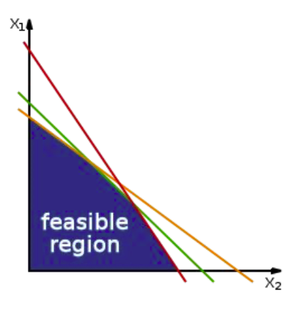
✔️ solution space
feasible region, fesible set, search space는 전부 solution space을 말하는 말이며 답이 될수 있는 모든 후보군들을 말하는 말이다. 이때, optimization문제라 하며는 이런 space에 정의된 답들 중 원하는 목표(최소, 최대)를 만들수 있는 답은 무었인가를 찾는 과정이다.

출처 및 참고자료: https://en.wikipedia.org/wiki/Feasible_region#:~:text=In_mathematical_optimization,_a_feasible,,_equalities,_and_integer_constraints.

✔️Time complexity
➡️ $f(x) \in O(g(x))$ as there exists c > 0(e.g. c = 1) and $x_0$ (e.g. $x_0$ = 5) such that $f(x) \leq cg(x)$ whenever $x \geq x_0$

출처 : Naver BoostCamp AI Tech - edwith 강의

✔️ $P$ , $NP$

문제의 클래스들을 지칭하며 $P$ 는 polynomial time에 끝나는 문제들을 지칭하는 반면 $NP$ 는 polynomial time안에 끝나지 않는 문제들을 지칭한다.
실생활에서는 $P$ , $NP$ 문제 이외에도 더 단순하게 끝나거나 아주 안끝나는 문제도 있지만 현실에서 마주하는 대부분의 문제는 $P$ , $NP$ 문제이고 $P$ 문제는 일반 알고리즘으로도 금방 풀지만 $NP$ , $NP-hard$ 문제( $NP$ 에 속하는 모든 문제에 대해 다른 문제)는 모든 요소를 고려하면 시간이 천문학적으로 오래 걸리기 때문에 ML모델을 이용하여 몇개의 Candidate를 이용하여 유망한 결과를 찾아나가는 식으로 수행을 한다.

✔️ Tradeoff

시간복잡도와 공간복잡도는 서로 tradeoff관계이다.
데이터 저장시에도 compress를 하지 않으면 공간이 많이 필요하나 찾는 시간은 덜 걸리게 된다. 반대로 compress를 하게 되면 공간은 비교적 덜 사용하나 찾는 시간은 오래 걸리게 된다.

⭐️ 이러한 관계를 잘 사용하는 것이 프로그래머로써 해야 할 일

✔️ Entroy(무질서도)
큐브를 예로 들면 처음에는(과거) 모든 면이 같은 색으로 맞춰진 큐브였으나 시간이 니자면(미래)색이 서로 흐트러진 상태가 되어진다.
➡️ 열역학 법칙에서도 사용이 되어지는 단어이며 시간이 흐르면 무질서도가 증가한다고 생각 할 수 있다.

✔️ ML은 세상에 있는 무질서한 데이터(미래)들을 정돈된 상태(과거)로 만드는 과정으로 이해 할 수 있다.
➡️ 내가 원하는 정보가 더 있는 상태로 바뀜

➡️ high entropy상태에서 데이터를 제공함으로써 low entropy상태로 변하게 해 준다.

동전의 엔트로피 예시

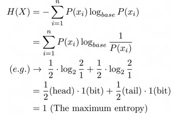
출처 : Naver BoostCamp AI Tech - edwith 강의

👉 base - 표현되어지는 경우의 수
👉 $\frac{1}{2}(head)$ , $\frac{1}{2}(head)$ - 앞, 뒷면이 나올 확률
👉 $1(bit)$ - 한 비트가 가지고 있을 수 있는 정보량

Parameter search

Parameter search, Hyperparameter search, Architecture search

✔️ 예전에는 사람이 model을 전반적으로 설계를 메뉴얼대로 building을 해 줘야 했다면 최근에는 ML이 영역을 확장하여 사람이 model building의 설계의 일부과정(hyperparameter 설정 등)에만 관여하여 building을 수행하는 형태로 바뀌어 가고 있고 미래에는 ML이 Architecture설계까지 영역을 확장하는 형태도 생각 해 볼 수 있다.

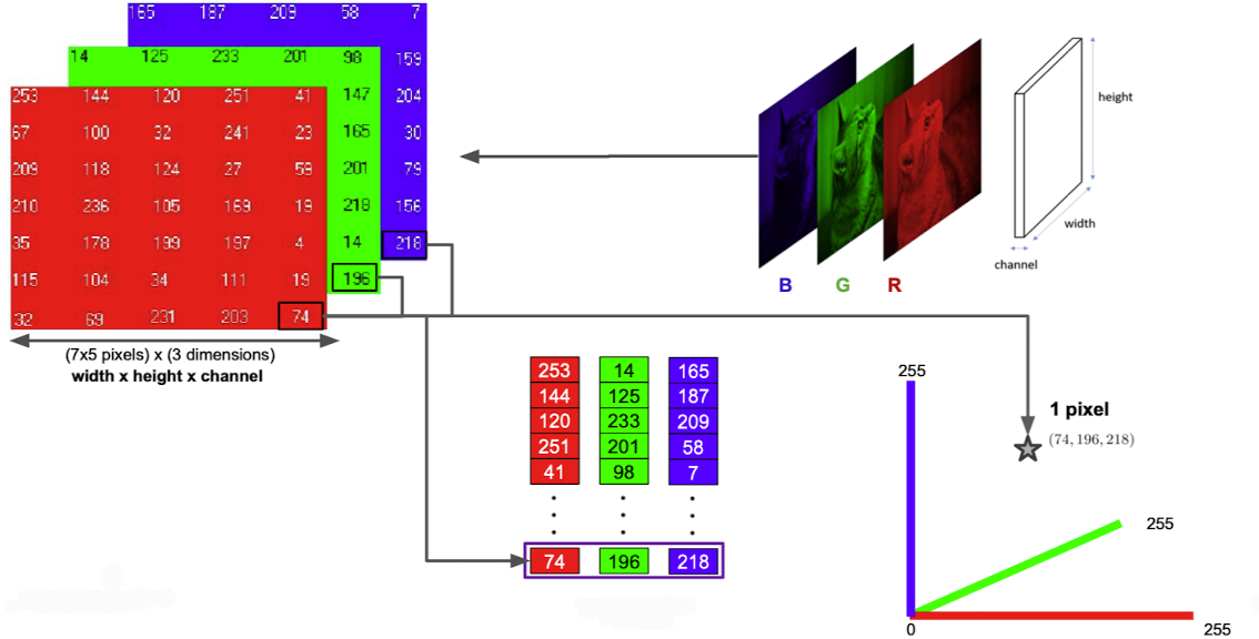
✔️ 현실의 것들은 데이터로 표현이 가능하고 데이터는 벡터로 표현이 가능하며 결정기인 ML모델로 Task를 수행하는 형태이다.

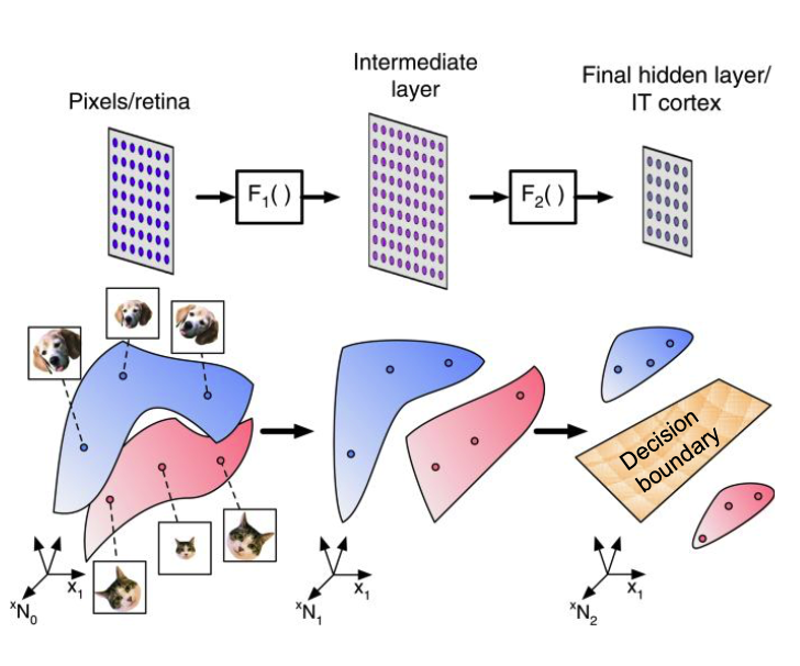
출처 : https://www.nature.com/articles/s41467-020-14578-5

출처 : Naver BoostCamp AI Tech - edwith 강의

RGB픽셀도 하나의 벡터로써 표현이 가능하다.

✔️ 다차원 공간의 Search space에서 optimal한 결과를 찾기 위해서는 귀납적 방법으로 유망한 값을 찾아나간다.(항상 최적의 값이라고 장담할 수는 없음)

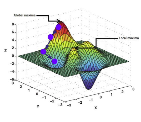
출처 : Naver BoostCamp AI Tech - edwith 강의

✔️ input,output데이터, Target데이터, weight( $w_1,w_2,...$ ) 심지어 neural network자체 또한 벡터의 한 점으로써 표현이 가능하다.

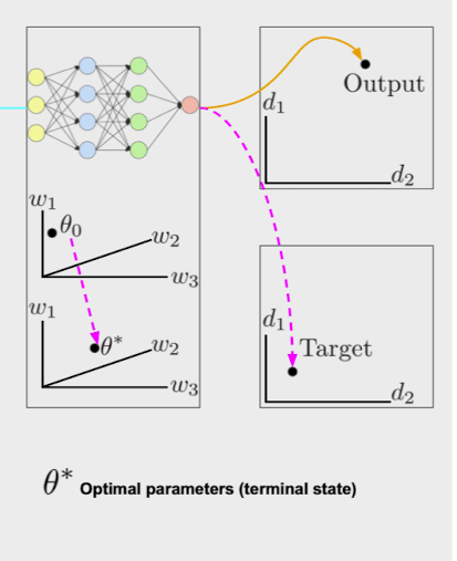
출처 : Naver BoostCamp AI Tech - edwith 강의

Hyperparameter search

✔️ Hyperparameter를 변경할때마다 모델이 다소 변화가 있고 모델 하나를 학습할 때 마다 큰 비용이 들어간다.

✔️ Grid search
hyperparameter설정을 할 때 어떠한 기준으로 설정을 할지에 대한 기준으로써 격자 모양으로 일정한 간격마다 경우의 수를 고려 해 줄 수도 있다.
Grid search의 단점은 조사하지 않은 사이에 최적의 답을 도출하는 조합이 있을수도 있기 때문에 Random Layout을 사용하기도 한다.

출처 및 참고자료 : https://www.sicara.ai/blog/2019-14-07-determine-network-hyper-parameters-with-bayesian-optimization

✔️ Surrogate Model
Hyperparameter를 input으로 가지고 output으로 실제 사용하고자 하는 모델의 결과를 가지고 학습을 진행하여 surrogate model학습을 진행함으로써 이 모델을 사용하여 Hyperparameter search을 진행

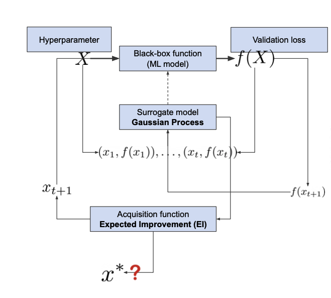
출처 : Naver BoostCamp AI Tech - edwith 강의

Gaussian process 논문 참고 - Figure1

https://arxiv.org/pdf/1012.2599.pdf?bcsi_scan_dd0fad490e5fad80=fwQqmV5CfHDAMm8dFLewPK+h1WGiAAAAkj1aUQ==&bcsi_scan_filename=1012.2599.pdf&utm_content=buffered388&utm_medium=social&utm_source=plus.google.com&utm_campaign=buffer

Neural Architecture search(NAS)

✔️ model을 compression한다?
아키텍쳐단의 이야기이지 param, hyperparam단의 얘기가 아님

✔️ 모델의 Goal
Performance향상만이 목표가 아닌 모델 size, co2 emission등 다양한 요건(multi-objective)을 만조해야 한다.

✔️ NAS는 multi-objective를 만족시키는 NAS(compression method)를 포함한 다양한 범주를 포함한다. => 사람이 만든 아키텍쳐가 아닌 NAS model이 아키텍쳐를 생성

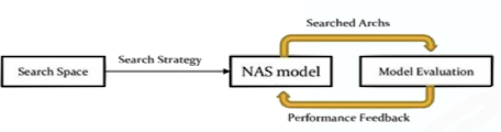
출처 : Naver BoostCamp AI Tech - edwith 강의

➡️ Search Strategy : 강화학습등의 방법으로 학습
어디를 Residual connection?, 어디랑 어디를 operation fuse할 것인가? , 어디랑 어디를 depthwise separation을 할지
➡️ Model이 다름 전략을 설정 : NAS
Search space에서 여러번 둘러보고 그 결과로 다양한 기형적인 아키텍쳐들을 볼 수 있음
참고 자료
https://arxiv.org/pdf/1611.01578.pdf

NAS for edge devices

✔️ edge device들을 위한 NAS의 종류

MnasNet
참고 자료
https://arxiv.org/pdf/1807.11626.pdf
👉 기본 컨셉은 직업 모바일에 넣어 모델을 돌려 실험을 해야 한다는 취지에서 model을 search space에서 sample하여 mobile device에 직접 넣어봄
👉 search space들 hierarchy하게 하여 sample -> setting을 다르게 하여 돌려봄(시간은 오래걸림)
PROXYLESSNAS
참고 자료
https://arxiv.org/pdf/1812.00332.pdf
👉 Differentiable NAS처럼 Model setting비용이 너무 커 Proxy기법을 썻었음(예전 NAS들) => 3,4레이어들만 학습하는 전체를 말고 일부만 학습 한다던지 등
👉 proxy task사용 시 아키텍쳐 최적화가 target task에 optimal함을 보장해주지 못하니 아예 쓰지 말자는 취지에서 나옴
ONCE-FOR-ALL
참고 자료
https://github.com/mit-han-lab/once-for-all
https://arxiv.org/pdf/1908.09791.pdf
👉 네트워크 한번 training시켜 여러가지 device상황에서(mobile 등) 약간만 바꿔 여기저기 적용시켜 보자
👉 retrain없이 약간만 바꿔 적용 -> 응용가능성에 초점
👉 이런 방법이 가능했던 것은 progressive shrinking방법 덕분(prunning과 관련이 있음)

💡 Regular convolution , depth wise separable convolution
👉 Regular convolution

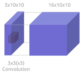
출처 : Naver BoostCamp AI Tech - edwith 강의

of computation : $3 * 3 * 3 * 16 * 10 * 10 = 43200$
(커널 크기 * 커널 크기 * input 채널 size * output channel size * feature map size)
👉 depth wise separable convolution

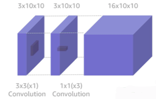
출처 : Naver BoostCamp AI Tech - edwith 강의

👉 각각 계산한 다음 합치자
👉 filter decompose분야이기도 함
of computation : $(3 * 3* 1) * 3 + (1 * 1 * 3) * 16 * 10 * 10 = 7500$
(커널 크기 * 커널 크기 * 중간 커널 수) * input 채널 size + (중간 커널 크기 * 중간 커널 크기 * input 채널 size) * output 채널 size

알뜰히

기본 컨셉 코드

dic = {'A' : 0, 'B' : 1, 'C': 2, 'D' : 3}
print("Codebook : ", dic)
string = "BCDADA"
print("Original message : {}, ({} bytes are needed)".format(string, len(string)))

# Encoding process
encoded = [dic[item] for item in [char for char in string]]
encoded = ''.join(map(str, encoded))
print("Encoded message message : {}, ({} bytes are needed)".format(encoded, len(encoded)/4)) # 0 ~ 3까지 2bit가 커버하기 때문
print("Compression rate : ", len(string)/ (len(encoded) / 4))

#Decoding process
reversed_dic = dict(map(reversed, dic.items()))
a = [item for item in list(encoded)]
decoded = [reversed_dic[int(num)] for num in [item for item in list(encoded)]]
decoded = ''.join(map(str, decoded))
print("Decoded message", decoded)

Codebook :  {'A': 0, 'B': 1, 'C': 2, 'D': 3}
Original message : BCDADA, (6 bytes are needed)
Encoded message message : 123030, (1.5 bytes are needed)
Compression rate :  4.0
Decoded message BCDADA

dic = {'A' : 0, 'B' : 10 , 'C' : 110, 'D' : 1110, 'E' : 11110, 'F' : 111110}
print("Codebook : ", dic)
string = 'DFEADEEDE'
print("Original message : {}, ({} bytes are needed)".format(string, len(string)))

# Encoding process
encoded = [dic[item] for item in [char for char in string]]
encoded = ''.join(map(str, encoded))
print("Encoded message message : {}, ({} bytes are needed)".format(encoded, len(encoded)/8))
print("Compression rate : ", len(string)/ (len(encoded) / 8))

# Decoding process
decoded = ''
temp = ''
inv_code = {v : k for k,v in dic.items()}
for c in encoded:
    temp += str(c)
    if int(temp) in inv_code.keys():
        decoded += inv_code[int(temp)]
        temp = ''
    else:
        pass

print("Decoded message : ", decoded)

Codebook :  {'A': 0, 'B': 10, 'C': 110, 'D': 1110, 'E': 11110, 'F': 111110}
Original message : DFEADEEDE, (9 bytes are needed)
Encoded message message : 111011111011110011101111011110111011110, (4.875 bytes are needed)
Compression rate :  1.8461538461538463
Decoded message :  DFEADEEDE

⭐️ 경량화에는 메모리 제약 또한 존재하기 때문에 정보를 효과적으로 압축하는 것 또한 매우 중요하다고 볼 수 있다.

압축(Compression)

✔️ 비손실 압축 VS 손실 압축

비손실 압축
압축된 자료를 복원하였을 때 그대로 원본이랑 동일하게 복원이 가능
(.zip, .png등)
손실 압축
압축된 자료를 복원하였을 때 그대로 원본이랑 동일하게 복원이 불가능
(.jpg, .mp3, .gif등)
예를 들어 mp3의 경우 사람이 들을 수 있는 소리 영역만 추출하여 압축하고 복원 시에는 원본에서 존재하는 사람이 듣지 못하는 영역의 소리는 복원하지 않는다.

✔️ Huffman coding(대표적인 압축 알고리즘)

string = "BCAADDCADCACFACE"

# Creating tree nodes
class NodeTree(object):
    def __init__(self, left = None, right = None):
        self.left = left
        self.right = right
    def children(self):
        return (self.left, self.right)
    def nodes(self):
        return (self.left, self.right)
    def __str__(self):
        return "%s %s" % (self.left, self.right)

# Main function implementing huffman coding
def huffman_code_tree(node, left = True, binString = ''):
    if type(node) is str:
        return {node : binString}
    (l,r) = node.children()
    d = dict()
    d.update(huffman_code_tree(l,True, binString + '0'))
    d.update(huffman_code_tree(r,False, binString + '1'))

    return d

# Calculating frequency
freq = {}
for c in string:
    if c in freq:
        freq[c] += 1
    else:
        freq[c] = 1

freq = sorted(freq.items(), key = lambda x : x[1], reverse= True)
nodes =  freq

while len(nodes) > 1:
    (key1, c1) = nodes[-1]
    (key2, c2) = nodes[-2]
    nodes = nodes[:-2]
    node = NodeTree(key1, key2)
    nodes.append((node, c1 + c2))
    nodes = sorted(nodes, key = lambda x : x[1], reverse = True)

huffmanCode = huffman_code_tree(nodes[0][0])
print(huffmanCode) # {'B': '000', 'E': '0010', 'F': '0011', 'D': '01', 'A': '10', 'C': '11'}

# Huffman encoding process
encoded = ''
for c in string:
    encoded += huffmanCode[c]

# Huffman decoding process
decoded = ''
temp = ''
inv_huffmanCode = {v:k for k, v in huffmanCode.items()}
for c in encoded:
    temp += c
    if temp in inv_huffmanCode.keys():
        decoded += inv_huffmanCode[temp]
        temp = ''
    else:
        pass


print("Encoded string : ", encoded)
print("Decoded string : ", decoded)
print("Original message : {} ({} bytes are needed)".format(string,len(string)))
print("Encoded message : {} ({} bytes are needed)".format(encoded, len(encoded)/ 8))
print("Compression rate : ", len(string) / (len(encoded)/ 8))

Encoded string :  0001110100101111001111011001110110010
Decoded string :  BCAADDCADCACFACE
Original message : BCAADDCADCACFACE (16 bytes are needed)
Encoded message : 0001110100101111001111011001110110010 (4.625 bytes are needed)
Compression rate :  3.4594594594594597

부호(Coding)

✔️ 일상적인 메세지( $M$ )과 일정한 부호로 변환한 메세지( ${M}'$ )이 있을 때 $len(M)$ > $len({M}')$ 일때, compression이라고 한다.(코딩의 부호화의 subset)

✔️ Finite State Machine(FSM)

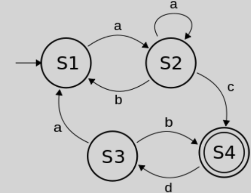
출처 : Naver BoostCamp AI Tech - edwith 강의
➡️ 유한번의 과정을 수행 후 끝이 나는 Machine(컴퓨터는 이런 Machine을 따르도록 만들어짐)

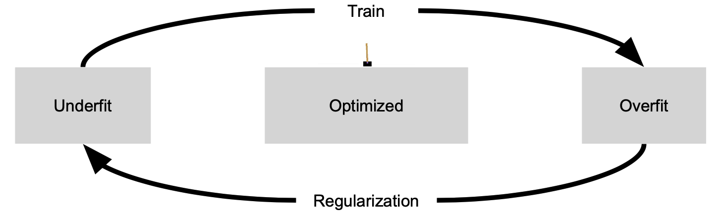
✔️ ML에서도 Underfit과 Overfit을 번걸아 가면서 Train과 Regularization을 수행하게 되고 FSM을 따라 종료가 되면서 Optimized된다.

출처 : Naver BoostCamp AI Tech - edwith 강의

✔️ Neural net은 데이터를 받고 encoding을 하여 input에 대한 새로운 데이더 값을 내놓게 된다.

✔️ 모든 데이터, model weight, model 자체 등도 하나의 벡터로써 표현이 가능하고 이 역시 encoding의 한 종류이다.

부호화(Encoding)

참고 자료
http://colah.github.io/posts/2015-09-Visual-Information/

출처 : Naver BoostCamp AI Tech - edwith 강의

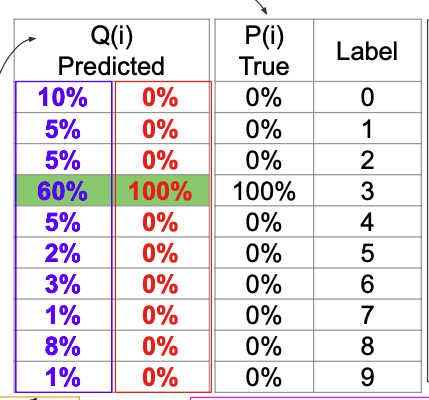
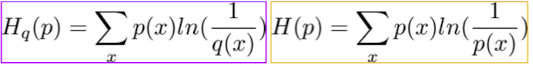
Classifier(Encoding)을 한 결과를 Q라하고 target을 P라 하자

출처 : Naver BoostCamp AI Tech - edwith 강의

Kullback–Leibler divergence으로써 두 분포거리에 대한 판단 지표로 사용(느낌은 이러하지만 대칭적이지는 않음 즉 , $P||Q$ 일때와 $Q||P$ 일때는 다르다.)

출처 : Naver BoostCamp AI Tech - edwith 강의

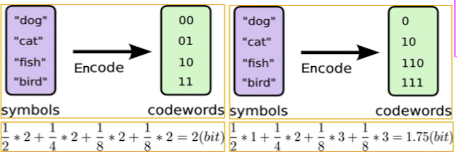
다음은 codebook과 symbol의 생성의 관점인데 오른쪽 그림처럼 어느 특정 단어가 많이 나온다면 그 부분의 symbol size를 작게 하고 적게 나오는 단어는 symbol size를 작게 해 주워 codebook을 구성하게 해 준다.

출처 : Naver BoostCamp AI Tech - edwith 강의

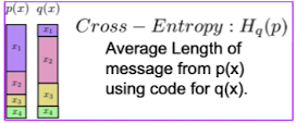
이때, cross-entropy는 q라는 codebook을 가지고 p라는 메세지를 encoding하였을 때의 무질서도로써 무질서도가 커진다는 이야기는 긴 encodig문자열이 나온다는 뜻과 같다. 즉, p라는 메세지는 p의 codebook을 사용했을 때 무질서도가 가장 낮다(0은 메제지가 아예 나오지 않는 경우를 제외하고는 존재하지는 않음)

출처 : Naver BoostCamp AI Tech - edwith 강의

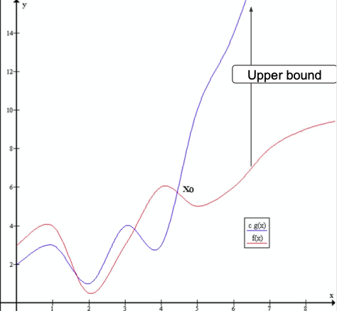
⭐️ 다시 Kullback–Leibler divergence를 보게 되면 cross-entropy는 entropy를 lower bound삼아서 무질서도를 낮추도록 network 학습이 진행된다.
참고 자료
http://colah.github.io/posts/2015-09-Visual-Information/

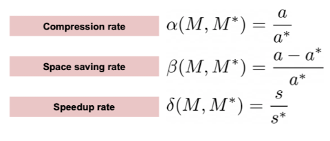
압축률(Compression rate)

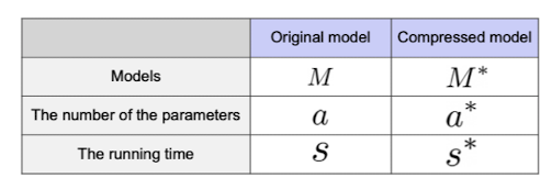
출처 : Naver BoostCamp AI Tech - edwith 강의

출처 : Naver BoostCamp AI Tech - edwith 강의

⭐️ 논문에서 pruning, quantization, huffmancoding등을 사용한 결과에 대한 성능 측정 지표로써 이러한 압축률등 여러 계산된 측정치들은 자주 사용이 됨을 볼 수 있다.

참고 자료
deep compression - https://arxiv.org/pdf/1510.00149

Reference

Naver BoostCamp AI Tech - edwith 강의

ganta

한걸음씩 꾸준히

이전 포스트

머신러닝 경량화 기초1

다음 포스트

머신러닝 경량화 기초2

딥러닝 이론

모델의 시공간

기본 컨셉 코드

space and time

Parameter search

Parameter search, Hyperparameter search, Architecture search

Hyperparameter search

Neural Architecture search(NAS)

NAS for edge devices

알뜰히

기본 컨셉 코드

압축(Compression)

부호(Coding)

부호화(Encoding)

압축률(Compression rate)

Reference

머신러닝 경량화 기초1

머신러닝 경량화 기초3

0개의 댓글