Building Large 3D Generative Models (2) - Model Architecture Deep Dive: VAE and DiT for 3D

Hwan Heo (허환)·2025년 7월 14일

3D 3D Generation 3d ai Clay Diffusion Transformer Generative Model Hi3DGen Hunyuan 3D Recitified Flow Rodin TripoSG VAE dit flow

3D AI

목록 보기

24/25

Figure from Hunyuan 3D 2.5

Related previous articles:

Introduction

지난 글 에서는 Large 3D Generative Model 을 구축하기 위한 첫 단계로, 데이터셋을 준비하고 필수적인 데이터 전처리 과정에 대해서 수학적, 위상학적 원리부터 실제 알고리즘 구현까지 심도 깊게 다뤄보았다.

이번 글에서는 3D Generative Pipeline 에서도 가장 core 에 해당하는 Shape Generative Model 의 구조를 본격적으로 파헤쳐보자.

이전 글들에서 간단하게 살펴본 것처럼 VAE 에서의 두 다른 접근 방식,

vecset-based
sparse voxel

에 대해서 VAE 부터 생성모델까지 자세하게 다뤄보도록 하겠다.

C. VAE Architecture

3D 데이터를 VAE로 압축하는 방식은 크게 두 가지로 나뉜다. 이 선택은 단순한 구현의 차이를 넘어, 3D 데이터를 어떻게 바라볼 것인가에 대한 근본적인 관점의 차이를 반영한다고 볼 수 있다.

Vecset-based VAE: 3D Shape 을 '순서 없는 점들의 집합' 으로 간주.
Sparse Voxel VAE: 3D Shape 을 '공간적 구조를 가진 3D 그리드' 로 간주.

이 두 가지 접근 방식이 어떻게 다른 아키텍처로 이어지는지, 비교 분석해보자.

C.1. VecSet VAE

From Mesh to an Unordered Set of Tokens

이름에서 알 수 있듯, vecset-based VAE는 3D Mesh를 벡터의 집합 (Vector Set), 즉 PointCloud 형태로 다룬다. 이 방식은 Mesh가 가진 1) 가변적인 꼭짓점 (vertex) 개수 문제와 2) Rotation/Translation Invariancy 를 자연스럽게 처리하기 위해 고안되었다.

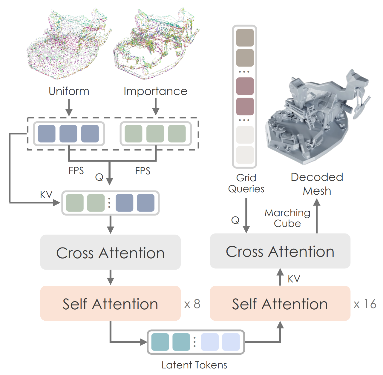
Figure: Hunyuan 3D 2.0's VAE. Sampling 된 pointcloud 이 fourier featuring 을 거쳐 Transformer Enc/Dec 를 통해 isosurface (SDF) 를 예측하도록 하는 vecset-based VAE architecture 를 보여준다.

Vecset-based VAE 의 latent encoding / decoding 과정은 비교적 간단하다:

Surface Point Sampling: Watertight Mesh 표면에서 고정된 개수 (e.g., 4096개)의 점을 샘플링
Fourier Feature Encoding: 샘플링된 각 점의 3D 좌표 ( $x, y, z$ )에 Positional Encoding (fourier featuring) 을 적용. 이는 모델이 절대 좌표가 아닌 점들 간의 상대적 위치 관계에 집중하게 하여 학습을 안정화시킨다.
Transformer Encoder: Fourier feature 이 적용된 point vector sequence 를 Transformer 블록에 통과시켜 점들 간의 전역적인 (global) 관계를 포착하고, 최종적으로 latent vector 를 예측한다.

이 방식의 핵심은 입력 데이터 단계에서 이미 3D structure 를 'Token Sequence' 로 변환한다는 것이다. VAE의 output 인 latent vector 또한 [Batch, Num_points, Latent_dim] 형태의 'tokenized' 점들의 집합이 되며, 이는 후속 생성 모델이 별도의 전처리 (patchfy) 없이 바로 데이터를 받을 수 있음을 의미한다.

그렇다면 이 과정이 실제 코드로 어떻게 구현되는지 상세히 들여다보자.

1. Encoder: PointCloud to Latent Vector

Encoder 의 목표는 pointcloud 를 VAE 가 다룰 수 있는 고정된 크기의 특징 vector sequence 로 압축 하는 것이다.

먼저, 3D 좌표 (x,y,z)에 Fourier featuring 을 적용한 후, 모든 점을 한 번에 처리하는 대신, FPS (Farthest Point Sampling) 로 추출된 소수의 대표 점들 (pointcloud_query) 을 Query 로, 전체 점들을 Key/Value 으로 삼아 Cross-Attention 을 수행한다. "이 대표 점들의 관점에서 전체 형상을 요약해 줘" 라는 의미로, 효율적인 정보 압축을 가능케 한다.

# vae/model.py : encode()

# ... FPS ...
fps_indices = data["fps_indices"]
pointcloud_query = torch.gather(pointcloud, 1, fps_indices.unsqueeze(-1).expand(-1, -1, pointcloud.shape[-1]))

# Perceiver: Cross-Attention
hidden_states = self.perceiver(pointcloud_query, pointcloud)

# Encoder: Self-Attention
for block in self.encoder:
    hidden_states = block(hidden_states)

Perceiver 를 통과한 feature 들은 여러 층의 Self-Attention 블록을 거치며 서로 정보를 교환하고, 최종적으로 3D 형태에 대한 고차원적인 관계를 학습하게 된다.

2. Bottleneck

VAE 가 단순한 auto-encoder 를 넘어 Generative AI 에서 sampling → 생성으로 이어지는 것은 bottleneck layer 의 DiagonalGaussianDistribution 클래스를 통한 ‘Reparameterization trick’ 에 있다.

# vae/utils.py

class DiagonalGaussianDistribution:
    def __init__(self, mean, logvar, deterministic=False):
        self.mean, self.logvar = mean, logvar
        self.std = torch.exp(0.5 * self.logvar)
        # ...

    def sample(self, weight: float = 1.0):
        # Reparameterization Trick
        sample = weight * torch.randn(self.mean.shape, device=self.mean.device)
        x = self.mean + self.std * sample
        return x

Encoder 가 출력한 feature vector (latent vector) 는 latent space 를 정의하는 mean 과 로그 분산 (logvar) 으로 변환된다. 이 값은 __init__에서 평균과 분산, 즉 latent space 에서의 '위치' 와 '불확실성의 정도' 를 정의한다.

여기서 핵심은 sample() method 에 구현된 Reparameterization Trick (Gaussian distribution 에서 noise 를 뽑아 mean, std 를 이용해 unnormalized 된 noise 를 생성) 이다. 이 기법 덕분에 미분 불가능한 '샘플링' 과정이 포함 됨에도 불구하고, 모델 전체에 걸쳐 Backpropagation 이 가능 해진다.

\epsilon ' = \mu + \sigma \cdot \epsilon, \quad \epsilon \sim N(0, I)

3. Decoder: Latent Vector to SDF

Decoder 의 목표는 압축된 latent vector 로부터, 우리가 원하는 임의의 3D 좌표의 SDF 값 을 알려주는 “continuous function" 를 만들어내는 것이다.

# vae/model.py : decode() & query()

def decode(self, latent: torch.Tensor):
    hidden_states = self.proj_up(latent)
    for block in self.decoder:
        hidden_states = block(hidden_states)
    return hidden_states

def query(self, query_points: torch.Tensor, hidden_states: torch.Tensor):
    # query_points: 3D coordinates
    query_points = self.fourier_encoding(query_points)
    query_points = self.proj_query(query_points)

    query_output = self.attn_query(query_points, hidden_states)
    pred = self.proj_out(query_output)
    return pred

decode()는 latent vector 를 이용해 SDF 값을 알고 싶은 3D coordinates (query_points) 에 대한 Cross-Attention을 수행하여 최종 SDF 값을 예측한다.

여기서 짚고 넘어갈 사안은, Vecset-based VAE 방식은 두 가지 어려운 문제 (Compression + Modality Conversion) 를 동시에 풀어야 하는 근본적인 부담을 안고 있다는 것이다.

Compression: 원본 메쉬를 대변하는 PointCloud 를 low-resolution latent vector 로 압축
Modality Conversion: discrete pointcloud → continuous 3D SDF 을 생성

이 과정에서 발생하는 문제들은 다음과 같다.

Sampling Error: 입력 단계에서 PointCloud 를 샘플링할 때, 원본 메쉬의 high-frequency details 정보가 영구적으로 손실된다 (sharp edge 나 복잡한 곡면의 정보 등).
Ill-posed Problem: Decoder 는 샘플링된 점과 점 사이의 "비어 있는 공간" 을 추론해야 함. 이는 정답이 하나로 정해져 있지 않은 ill-posed problem 이다.
Smoothing Effect: 모델이 학습하는 loss function 가 보통 L1/L2 norm 기반의 Reconstruction Loss 이기 때문에, sharp features 들은 자연스럽게 smoothing 되어 뭉개진다.
Reconstruction Error (Quantization Error): 최종적으로 이 모든 추론을 거쳐 만들어낸 연속적인 SDF 함수를 다시 discreate voxel grid 에 샘플링하여 mesh 를 추출하는 과정에서 Quantization Error 가 발생하며, 디테일이 한 번 더 손실된다.

Summary

VecSet VAE: 3D 를 token sequence 로 변환. latent 도 [B, N, C] 형태의 token sequence -> DiT 모델 설계시 patchfy 가 필요 없다.

입력 정보의 손실 (Sampling Error) 과 출력 정보의 손실 (Quantization Error) 이라는 양쪽의 정보 손실을 겪으며, 그 사이의 간극을 메우는 어려운 추론 문제 (Ill-posed Problem) 까지 풀어야한다.

C.2. Sparse Voxel VAE

3D as a Spatial Grid

반면, Sparse Voxel VAE는 3D 데이터를 2D 이미지의 확장판, 즉 3D 공간 그리드 (Grid)로 취급한다. Trellis 와 같은 모델에서 사용하는 이 방식은 U-Net 과 비슷한 3D Convolutional Network 구조를 차용한다.

이 접근법의 핵심은 3D 형태를 공간적 구조가 명확한 텐서 로 다루는 데 있다. Sparse-voxel 기반의 VAE 모델들은 Transformer 대신 Convolution 연산을 통해 local 특징과 hierarchical 구조를 학습하게 된다.

1. Encoder

인코더는 입력으로 들어온 3D 그리드 ([B, C, D, H, W])를 ResBlock3d와 DownsampleBlock3d(3D Convolution 또는 3D Pooling) 를 통해 점진적으로 다운샘플링한다.

# Trellis/models/sparse_structure.py

class SparseStructureEncoder(nn.Module):
    def __init__(self, in_channels: int, latent_channels: int, channels: List[int], ...):
        super().__init__()
        # Input Layer
        self.input_layer = nn.Conv3d(in_channels, channels[0], 3, padding=1)

        # Downsampling Blocks
        self.blocks = nn.ModuleList([])
        for i, ch in enumerate(channels):
            self.blocks.extend([ResBlock3d(ch, ch) for _ in range(num_res_blocks)])
            if i < len(channels) - 1:
                self.blocks.append(DownsampleBlock3d(ch, channels[i+1]))

        # Bottleneck
        self.middle_block = nn.Sequential(...)
        self.out_layer = nn.Sequential(..., nn.Conv3d(channels[-1], latent_channels*2, 3, padding=1))

    def forward(self, x: torch.Tensor, ...):
        # x: [B, C, D, H, W], a 3D grid
        h = self.input_layer(x)
        for block in self.blocks:
            h = block(h) # Convolutions and Downsampling

        h = self.middle_block(h)
        h = self.out_layer(h)

        mean, logvar = h.chunk(2, dim=1) # 채널을 반으로 나눠 mean, logvar로 사용
        # ... Reparameterization Trick ...
        return z # Latent z is also a 3D grid: [B, latent_C, D', H', W']

이 코드는 전형적인 3D U-Net 의 Encoder 구조와 사실상 동일하다. ResBlock3d는 3D Convolution 과 Skip-connection 을 통해 이루어져 feature representation 을 효과적으로 배우고, DownsampleBlock3d는 stride=2인 convolution 을 이용해 spatial dimension (D, H, W) 을 절반으로 줄이는 대신, feature dimenstion (C)을 늘려 정보를 압축한다.

주목할 점은, forward 함수의 마지막 부분이다. 최종 출력인 h의 채널을 반으로 나누어 각각 평균 (mean) 과 로그 분산 (logvar) 으로 사용한다. 즉, 최종 출력인 잠재 표현 z 또한 [B, latent_C, D', H', W'] 형태의 작은 'Latent Grid' 라는 점이다. 이는 Vecset-based VAE 가 vector sequence 를 출력하는 것과 근본적으로 다른 지점이다. Latent representation 자체가 공간적 구조를 유지하고 있는 것이다.

2. Decoder: Feature Upsampling

Decoder 는 Encoder 와 완벽한 대칭 구조를 이룬다. 압축된 'Latent Grid' 를 입력받아, UpsampleBlock3d를 통해 점진적으로 원래의 3D Grid resolution 으로 복원한다.

# Trellis/models/sparse_structure.py

class UpsampleBlock3d(nn.Module):
    def __init__(self, in_channels: int, out_channels: int, mode: Literal["conv", "nearest"] = "conv"):
        # ...
        if mode == "conv":
            self.conv = nn.Conv3d(in_channels, out_channels*8, 3, padding=1)

    def forward(self, x: torch.Tensor) -> torch.Tensor:
        # ...
        x = self.conv(x)
        return pixel_shuffle_3d(x, 2) # (D,H,W) -> (2D,2H,2W)

class SparseStructureDecoder(nn.Module):
    def __init__(self, out_channels: int, latent_channels: int, ...):
        super().__init__()
        self.input_layer = nn.Conv3d(latent_channels, channels[0], 3, padding=1)
        self.middle_block = nn.Sequential(...)
        self.blocks = nn.ModuleList([])
        # ... Upsampling Blocks ...

    def forward(self, x: torch.Tensor) -> torch.Tensor:
        # x: Latent Grid [B, latent_C, D', H', W']
        h = self.input_layer(x)
        h = self.middle_block(h)
        for block in self.blocks:
            h = block(h) # Convolutions and Upsampling
        h = self.out_layer(h)
        return h # Reconstructed Grid [B, C, D, H, W]

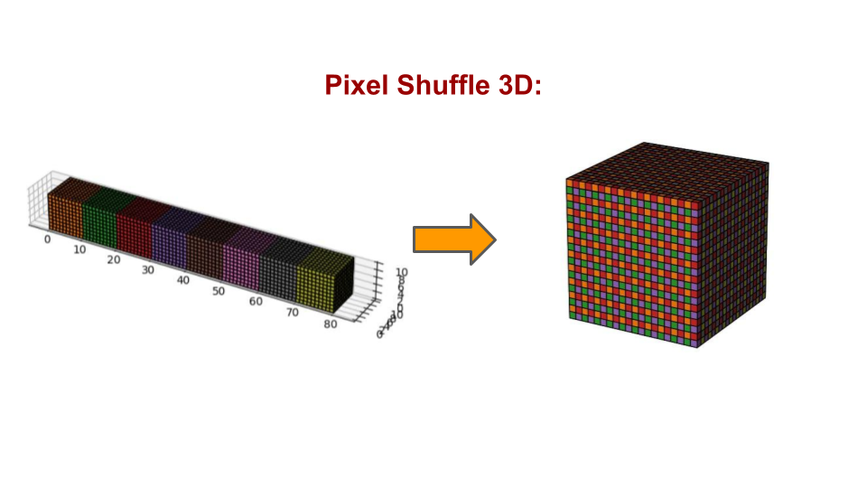
UpsampleBlock3d 는 pixel_shuffle_3d 기법을 사용한다. 이는 3D Transposed Convolution 과 유사한 역할을 하지만, 연산 효율성과 checkerboard artifacts 방지 측면에서 더 유리하다고 알려져 있다. 이는 3D Transposed Convolution 이 가진 잠재적인 문제점들을 피하면서도, 효율적으로 공간 해상도를 높이는 매우 효과적인 대안이다.

def pixel_shuffle_3d(x: torch.Tensor, scale_factor: int) -> torch.Tensor:
    """
    3D pixel shuffle.
    """
    # 1. init state
    B, C, H, W, D = x.shape

    # 2. Channel Decomposition
    C_ = C // scale_factor**3
    x = x.reshape(B, C_, scale_factor, scale_factor, scale_factor, D, H, W)

    # 3. Dimension Re-Permutation 
    x = x.permute(0, 1, 5, 2, 6, 3, 7, 4) # (B, C_, H, scale_d, W, scale_h, D, scale_w)

    # 4. Reshaping
    x = x.reshape(B, C_, H*scale_factor, W*scale_factor, D*scale_factor)

    return x

scale_factor=2 일 때, x의 초기 shape이 [B, 8C', H, W, D] 라고 생각해보자 (UpsampleBlock3d에서 out_channels*8을 한 이유가 바로 이것).

pixel_shuffle_3d kernel 은 downsampling 과 반대로 channel dim 을 줄이면서, spatial dim 을 2배씩 늘리는 연산을 수행한다.

즉,

x = x.reshape(B, C_, scale_factor, scale_factor, scale_factor, D, H, W)
x = x.permute(0, 1, 5, 2, 6, 3, 7, 4)

을 통해 텐서의 차원 순서를 뒤섞어 (shuffle), channel dimenstion 에 있던 spatial information 을 실제 spatial dimenstion 차원 옆으로 가져온다.

permute 이전: (B, C', scale_h, scale_w, scale_d, H, W, D) (논리적 순서)
permute 이후: (B, C', H, scale_h, W, scale_w, D, scale_d)

이제 각 spatial dimenstion (H, W, D) 바로 뒤에, 그 공간을 확장시킬 scale_factor가 위치하게 되어, 메모리 상에서 데이터의 순서가 재배열되었다. 이후 reshape 을 통해 인접한 차원들을 하나로 합쳐주어, (H, scale_h)는 H*2로, (W, scale_w)는 W*2로, (D, scale_d)는 D*2로 합쳐진다.

결과적으로, [B, 8C', H, W, D] 였던 tensor 는 채널이 C'로 줄어든 대신, 공간 해상도가 [B, C', 2H, 2W, 2D]로 2배씩 커진 tensor 로 변환된다.

왜 Transposed Convolution보다 나은가?

연산 효율성: pixel_shuffle은 주로 메모리 재배열 연산(reshape, permute)으로 이루어져 있어 계산 비용이 매우 저렴하다. 주된 연산은 그 이전에 수행되는 단 한 번의 일반 Conv3d 뿐이다.
Checkerboard Artifacts: Transposed Convolution은 커널이 겹치는 방식 때문에, 출력 결과물에 마치 체스판 같은 격자무늬 노이즈가 생기는 고질적인 문제가 있다. 이는 특히 생성 모델에서 시각적 품질을 크게 저하시킨다. pixel_shuffle은 커널 오버랩 없이 각 픽셀이 독립적으로 계산된 후 재배치되므로, 이러한 아티팩트가 발생하지 않는다.
학습 안정성: 더 간단하고 직접적인 연산은 그래디언트 흐름을 원활하게 하여 학습을 더 안정적으로 만드는 경향이 있다.

vs. VecSet-Based VAE

앞서 VecSet-baed VAE 가 가진 여러가지 문제점을 기억하는가? Sparse-Voxel 기반 VAE 의 장점은 vecset-based 와 비교할 때 명확하다.

No Sampling Error: 입력 자체가 원본 메쉬의 전체적인 기하학 정보를 담고 있는 SDF 그리드이므로, 샘플링으로 인한 정보 손실이 없다. (물론, 최초 전처리 단계에서의 양자화 오류는 존재하지만, 이는 VAE 모델의 학습 범위 밖)
Well-posed Problem: 모델은 "점과 점 사이를 추론" 하는 어려운 문제를 풀 필요가 없다. 그저 "SDF 그리드를 SDF 그리드로" 복원하는, 즉 동일한 modality 내에서의 압축 및 복원 문제에만 집중하면 된다.
No Modality Conversion Burden: 입력과 출력의 형태가 같으므로, VAE 는 오직 정보의 효율적인 압축과 복원에만 집중.

결론적으로 이를 요약하면 다음과 같다.

"Vecset-based VAE는 정보 손실과 어려운 추론 문제를 동반하는 'Modality Conversion + Compression' 모델인 반면, Sparse Voxel VAE 는 훨씬 더 잘 정의된 'Compression' 모델이다."

이러한 근본적인 차이 때문에, shape preservation 과 detail reconstruction 측면에서는 Sparse Voxel VAE 가 구조적으로 훨씬 더 유리한 고지에 서 있다고 할 수 있다. Vecset-based 접근법의 장점은 입력 데이터의 유연성 (메쉬가 아닌 포인트 클라우드도 바로 처리 가능) 에 있지만, 고품질의 3D 형태를 생성하는 데에는 더 많은 구조적 한계를 가지는 것이 사실이다. 이는 최근 Sparse-Voxel 기반 연구들의 약진으로 증명되고 있는데, [Section E] 에서 이에 대해 좀 더 깊게 논의해보도록 하겠다.

Summary

Sparse Voxel VAE: 3D 의 spatial grid structure 를 유지. latent 도 [B, C, D, H, W] 형태의 3D grid -> DiT 설계 시 3D 에 대한 Patchfy 필요하다.

Vecset-based VAE 가 겪는 modality conversion 문제를 겪지 않기 때문에 유연한 확장성을 지닌다.

D. Shape Generative Model: DiT on Latent Space

이제 VAE가 만들어낸 두 종류의 latent space 위에서, DiT 기반 생성 모델이 어떻게 다르게 설계되는지 살펴보자.

D.1. Diffusion Transformer

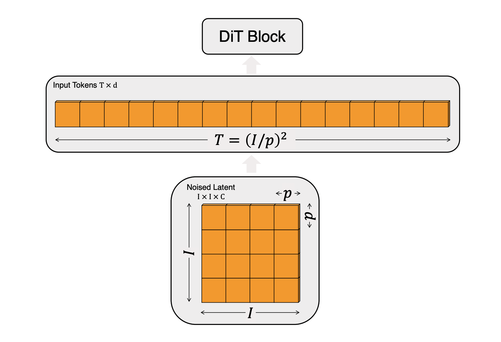
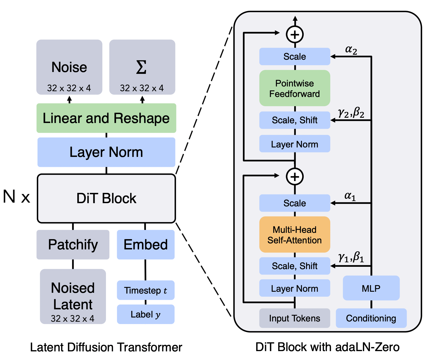
2D 이미지 생성에서 DiT의 혁신은 Vision Transformer(ViT)의 방법론을 차용한 것에서 시작한다. ViT는 이미지를 일정한 크기의 패치(Patch)로 자르고, 각 패치를 하나의 토큰(Token)으로 간주하여 Transformer의 입력 시퀀스로 사용한다.

원본 2D DiT 코드를 살펴보면 이 과정이 명확하게 드러나는데,

# From Original DiT by Facebook Research
class DiT(nn.Module):
    def __init__(self, input_size=32, patch_size=2, ...):
        super().__init__()
        # ...
        self.x_embedder = PatchEmbed(input_size, patch_size, in_channels, hidden_size, bias=True)
        # ...

    def forward(self, x, t, y):
        # x: (N, C, H, W) tensor of spatial inputs (images)
        # The first step is to patchify the image `x`
        x = self.x_embedder(x) + self.pos_embed  # (N, T, D), T = num_patches
        # ...

x_embedder 는 nn.Conv2d 를 이용해 이미지를 패치로 나누고, 각 패치를 linear transform 하여 (N, T, D) 형태의 token sequence 를 만든다. 즉, 공간적 Grid 데이터를 token sequence 로 변환하는 Patchify 과정이 필수적이다.

이를 명확히 인지하고 이후 3D 에서의 DiT 들이 어떻게 설계되어 있는지 살펴보겠다.

D.2. VecSet DiT

이전 단계에서 vecset-based VAE를 통해 3D Mesh를 vecset-based latent, 즉 PointCloud 형태의 잠재 latent vector 로 변환한 것을 상기해보자. 이 데이터의 형태는 [Batch, Num_points, Latent_dim] 이다.

즉, Vec-set VAE의 출력물은 이미 [B, N, C] 형태의 token sequence 이다. 따라서 DiT 는 이 시퀀스를 바로 처리할 수 있으며, 2D 이미지 DiT에서 필요했던 Patchify 과정이 필요 없어진다.

이 경우에 DiT model 은 feature dimension 만 맞춰주는 간단한 linear layer 정도를 제외하면, cross-attention 과 self-attention 으로 이루어진 일반적인 Transformer block 의 집합으로 간단하게 이루어진다.

# DiT w/ vecset-based VAE
# ...
class DiTLayer(nn.Module):
    def __init__(self, dim, num_heads, qknorm=False, gradient_checkpointing=True, qknorm_type="LayerNorm"):
        super().__init__()
        self.dim = dim
        self.num_heads = num_heads
        self.gradient_checkpointing = gradient_checkpointing

        self.norm1 = nn.LayerNorm(dim, eps=1e-6, elementwise_affine=False)
        self.attn1 = SelfAttention(dim, num_heads, qknorm=qknorm, qknorm_type=qknorm_type)
        self.norm2 = nn.LayerNorm(dim, eps=1e-6, elementwise_affine=False)
        self.attn2 = CrossAttention(dim, num_heads, context_dim=dim, qknorm=qknorm, qknorm_type=qknorm_type)
        self.norm3 = nn.LayerNorm(dim, eps=1e-6, elementwise_affine=False)
        self.ff = FeedForward(dim)
        self.adaln_linear = nn.Linear(dim, dim * 6, bias=True)
   # ...

class DiT(nn.Module):
    def __init__(self, latent_dim=8, hidden_dim=1024, ...):
        super().__init__()
        # No PatchEmbed layer, but projection linear layer!
        self.proj_in = nn.Linear(latent_dim, hidden_dim) # Simple projection
        # timestep encoding
        self.timestep_embed = TimestepEmbedder(hidden_dim)

        # transformer layers
        self.layers = nn.ModuleList(
            [DiTLayer(hidden_dim, num_heads, qknorm, gradient_checkpointing, qknorm_type) for _ in range(num_layers)]
        )

        # project out
        self.norm_out = nn.LayerNorm(hidden_dim, eps=1e-6, elementwise_affine=False)
        self.proj_out = nn.Linear(hidden_dim, latent_dim)
    # ...

경우에 따라서는 pointcloud sampling 자체가 token sampling 의 의미를 내포하고 있다고 해석할 수도 있겠다.

D.3. Sparse Voxel DiT

반면, Sparse Voxel VAE의 출력은 [B, C, D, H, W] 형태의 3D Latent Grid 이다. 이 공간적 구조를 가진 데이터를 Transformer가 처리하기 위해서는, 2D DiT와 마찬가지로 Patchify 과정이 다시 필요해진다.

# From Trellis (Voxel-based)
class SparseStructureFlowModel(nn.Module):
    def forward(self, x: torch.Tensor, ...):
        # x: [B, C, D, H, W], a 3D grid latent space
        h = patchify(x, self.patch_size) # Patchify the 3D grid
        h = h.view(*h.shape[:2], -1).permute(0, 2, 1).contiguous()
        h = h + self.pos_emb[None] # Add 3D positional embeddings
        # ... Transformer blocks process the token sequence ...
        h = unpatchify(h, self.patch_size) # Unpatchify back to a grid
        return h

3D Voxel Grid x를 3D patch 로 나누고, 이를 token sequence 로 변환하여 Transformer에 입력한다.

Trellis 의 patchfy 함수:

def patchify(x: torch.Tensor, patch_size: int):
    """
    Patchify a tensor.

    Args:
        x (torch.Tensor): (N, C, *spatial) tensor
        patch_size (int): Patch size
    """
    DIM = x.dim() - 2
    for d in range(2, DIM + 2):
        assert x.shape[d] % patch_size == 0, f"Dimension {d} of input tensor must be divisible by patch size, got {x.shape[d]} and {patch_size}"

    x = x.reshape(*x.shape[:2], *sum([[x.shape[d] // patch_size, patch_size] for d in range(2, DIM + 2)], []))
    x = x.permute(0, 1, *([2 * i + 3 for i in range(DIM)] + [2 * i + 2 for i in range(DIM)]))
    x = x.reshape(x.shape[0], x.shape[1] * (patch_size ** DIM), *(x.shape[-DIM:]))
    return x

VAE 단에서 유지했던 공간 정보가 Transformer의 입력 단계에서 sequence 로 변환되는 것!
즉 Trellis 의 DiT 는 2D DiT 의 3D 로의 확장 버젼이라고 볼 수 있다.

Figure from Scalable Diffusion Models with Transformers

D.4. Training with Rectified Flow

이제 이 DiT를 어떻게 학습시키는지 알아보자.

앞선 글에서 언급했듯, 최근 3D Generative Pipeline에서 이 Shape 생성 모델들은 Rectified Flow 프레임워크 위에서 동작한다.

Source ( $z_0 \sim p_0$ ): source distribution (일반적으로 standard normal distribution $\mathcal{N}(0, I)$ )
Target ( $z_1 \sim p_1$ ): target distribution (데이터의 latent space distribution $q_{data}$ ) 의 target 샘플

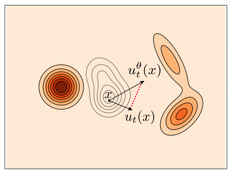
여기서 모델 학습의 objective 는 source distribution 으로부터 target distribution 까지의 변환 경로 를 예측하는 것이다.

특히 Rectified Flow 은 시간 $t \in$ 에 따라 변하는 확률 분포의 경로 $p_t$ 를 정의하고, 이 경로를 가장 간단한 형태인 linear interpolation 으로 가정한다.

z_t = (1-t)z_0 + t z_1

이 경로 위의 특정 시점 $t$ 의 한 점 $z_t$ 가 주어졌을 때, 모델 (DiT)의 역할은 이 직선 경로의 velocity vector 를 예측하는 것이다. 이 경로의 velocity 는 시간 $t$ 에 대해 미분하여 구할 수 있으며,

v_t = \frac{d z_t}{dt} = z_1 - z_0

위와 같이 이 velocity 는 시간 $t$ 나 위치 $z_t$ 에 관계없이 항상 상수 벡터인 $v = z_1 - z_0$ 가 된다. 따라서, 모델 $v_\theta(z_t, t)$ 는 현재 위치 $z_t$ 와 시간 $t$ 가 주어졌을 때, 이 constant velocity vector $z_1 - z_0$ 를 예측하도록 학습 된다.

위의 내용을 일반적인 형태의 Objective Function 으로 정리하면 그것이 곧 흔히 일컫는 Conditional Flow Matching (CFM) Loss 이 되는 것을 알 수 있다.

\mathcal{L}_{CFM}(\theta) = \mathbb{E}_{t \sim U(0,1), z_0 \sim p_0, z_1 \sim p_1} \left[ || v_\theta(z_t, t) - (z_1 - z_0) ||^2 \right]

이것이 바로 Rectified Flow의 핵심 아이디어이다.

실제 3D Flow Matching model 의 training_step 코드 또한 이 CFM 의 아이디어를 충실히 반영하여 구현하고 있다.

# From Model.training_step
def training_step(self, data, iteration):
    # ...
    # 1. Get Condition `c` from image
    cond = self.get_cond(cond_images.view(-1, C, H, W), cond_num_part)

    with torch.no_grad():
        # 2. Get Target Latent `z_1` from VAE
        # posterior = self.vae.encode(data)
        latent = posterior.mode().float().nan_to_num_(0)  # z_1

        # 3. Create a point `z_t` on the straight path
        #    z_t = t*z_1 + (1-t)*z_0, where z_0 is noise
        noisy_latent, noise, timesteps = self.scheduler.add_noise(
            latent, self.config.logitnorm_mean, self.config.logitnorm_std
        ) # noisy_latent is z_t, noise is z_0

    # 4. Predict the velocity vector with DiT
    noisy_latent = noisy_latent.to(dtype=self.precision)
    model_pred = self.dit(noisy_latent, cond, timesteps)

    # 5. Calculate Loss
    # The velocity vector v = z_1 - z_0 = latent - noise
    # The code uses target = noise - latent, which is -v. This is also a valid objective.
    target = noise - latent
    loss = F.mse_loss(model_pred.float(), target.float())

    return output, loss

Condition: 입력 이미지에서 DINOv2 feature 를 추출하여 이미지 조건 $c$ 를 만듬
Target $z_1$ : pre-trained VAE를 이용해 Ground Truth 3D 데이터로부터 latent ( $z_1$ )를 인코딩
Trajectory $z_t$ : scheduler.add_noise 함수가 시간 $t$ 를 랜덤 샘플링하고, $z_t = t \cdot z_1 + (1-t) \cdot z_0$ 공식을 이용해 노이즈 $z_0$ 와 타겟 $z_1$ 사이의 한 점 noisy_latent ( $z_t$ )를 생성
Velocity Estimation: DiT 모델 $v_\theta$ 는 $z_t$ , 조건 $c$ , 시간 $t$ 를 입력받아 속도 벡터(의 반대 방향)를 예측 (model_pred)
Loss: 예측된 속도 model_pred와 실제 속도 target 사이의 MSE Loss를 계산하여, 위에서 정의한 $\mathcal{L}_{CFM}$ 을 최소화

Diffusion 모델의 복잡한 score-matching 목적 함수 대신, "직선 경로의 방향을 예측하라"는 매우 간단하고 명확한 MSE Loss를 사용함으로써 빠르고 안정적인 학습을 가능하게 한다.

이 Rectified Flow 및 Flow Matching 에 대한 물리적, 수학적 자세한 설명은 다음을 참고: From Flow Matching to Optimal Transport: A Physics-based View of Generative Models

Flow 에 대한 수학적 정의들과, 왜 Rectified Flow 가 직선 경로를 선택하는지에 대해 물리학적으로 (Optimal Transport, Least Action Principle) 연관지어 설명한다.

E. Discussion: Semantic vs. Spatial

지금까지 우리는 3D 생성에 대한 VAE 와 DiT architecture, 그리고 학습 방법론을 상세히 분석했다. 여기서 한 걸음 더 나아가, 3D 생성 모델의 발전 방향에 대해 최근 research community 가 던지고 있는 화두에 대해서 얘기해보자.

"과연 좋은 3D 생성 모델을 만들기 위해 우리는 무엇을 정렬(align)해야 하는가? Vision Foundation Model (2D) 의 Semantic Structure인가, 아니면 3D 고유의 Spatial Structure인가?"

E.1. The Reconstruction vs. Generation Dilemma

최근 2D 이미지 생성 분야에서 발표된 VA-VAE (Vision-Aligned VAE) 연구는 중요한 observation 을 제시한다.

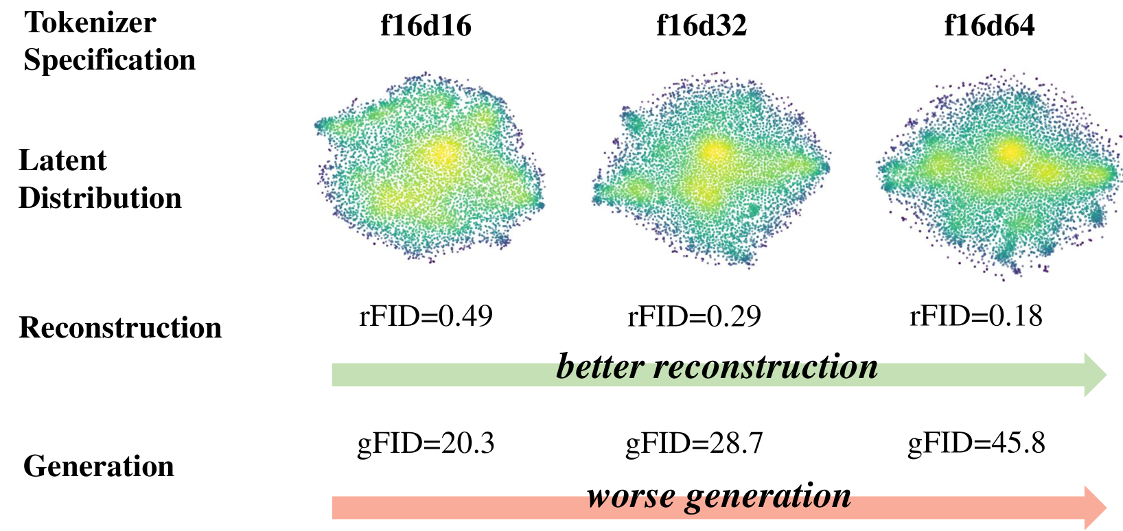
VAE 의 latent space 이 높은 차원을 가질수록 원본 이미지 복원 (Reconstruction) 품질은 향상되지만, 이 복잡한 latent space 위에서 학습해야 하는 생성 모델 (DiT) 의 성능은 오히려 저하된다.

왜 이런 현상이 발생할까? 저자들은 높은 reconstruction quality 만을 목표로 학습된 VAE의 latent space 이 의미론적으로 잘 구조화되어 있지 않기 때문이라고 주장한다.
즉, 잠재 공간 내의 벡터들이 무질서하게 흩어져 있어, 생성 모델이 '고양이'와 같은 특정 개념을 학습하기 매우 어렵다는 것.

VA-VAE의 해결책은 simple yet effective 한데, VAE의 latent space 를 Vision Foundation Model (e.g., DINO)의 feature space 와 align 시키는 것이다. VAE 학습 시, latent vector 와 DINO featur vector 간의 cosine similarity 를 높이는 loss 추가하는 것만으로, latent space 에 다음과 같은 이점이 생긴다.

Semantically Rich & Well-structured: Semantically 유사한 객체들이 latent space 에서도 가깝게 모임
Faster Convergence: Semantic 단위로 sturctured 된 latent space 덕분에, DiT는 low-level 의 픽셀 조합이 아닌, high-level semantic 단위 간 관계 학습에 집중할 수 있게 되어 학습 속도가 비약적으로 빨라진다.
(VA-VAE: 1400 epoch → 80 epoch)

E.2. VA-VAE and 3D Generation

Vecset-based VAE는 Point Cloud 를 이용해 3D shape 의 reconstruction 에만 초점을 맞춘, VA-VAE 가 지적한 'Reconstruction 특화' VAE와 유사한 측면이 있다. 이는 DiT (Flow Model) 가 input condition (2D) 에 맞는 Shape 을 생성하기 위해, 구조화되지 않은 넓은 latent space 을 비효율적으로 탐색해야 하므로 수렴이 느리며 성능이 제한될 수 있다는 가설 로 이어진다.

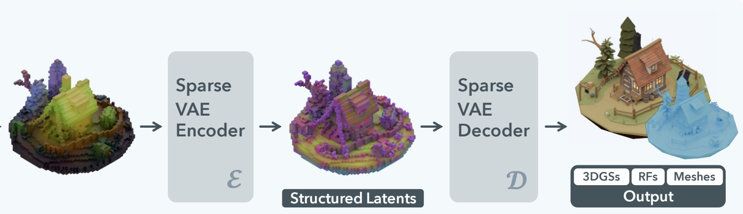
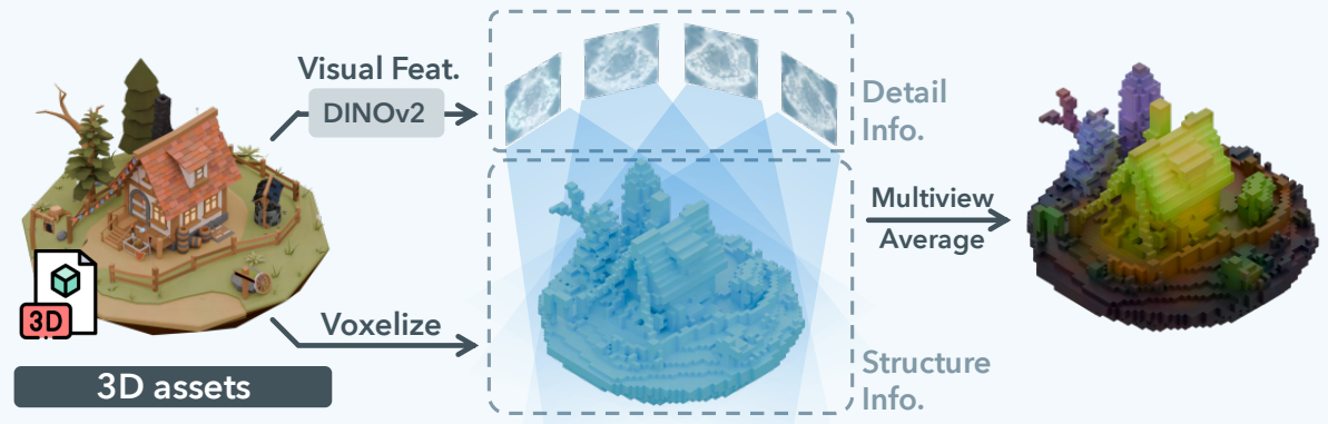
반면 Trellis는 이미 VA-VAE 와 유사한 아이디어를 3D 에서 SLAT (Structured Latent)이라는 개념으로 구현했다고 볼 수 있다. SLAT 은 DINO feature map 그 자체를 VAE 의 학습 목표로 삼아, 공간적 구조를 가진 의미론적 latent space 를 만든다. 즉, "DINO가 이미 충분히 좋으니, 이를 그대로 3D 공간에 매핑해서 쓰자!"는 접근인 셈.

하지만 이 방식은 VAE 의 latent space 를 사실상 두 개로 쪼개서 구성한다는 문제가 있다. 즉, '어디에 형태가 존재하는가?' 를 결정하는 Structure 와, '그곳에 무엇이 있는가?' 를 결정하는 Feature 로 구성된다는 것. 이로 인해 생성 과정은 복잡한 2-stage 파이프라인으로 분리된다.

1) Structure Generation: 먼저, 어떤 복셀이 activated 를 결정하는, 즉 Sparse Structure 의 indices 생성해야 한다. Trellis는 이를 위해 별도의 Conditional Flow Matching (CFM) 모델을 학습시킨다.
2) Feature Generation: 1단계에서 생성된 Sparse Structure 를 조건으로 하여, 두 번째 모델 (DiT-like Transformer) 이 각 activated voxel 위치에 해당하는 SLAT, 즉 projected DINO feature 를 생성한다. 이 모델의 학습 목표는 'Gaussian Noise → 해당 voxel 의 projected DINO feature' 라는 매우 복잡한 mapping 관계다.

이로 인해 VAE 는 이제 단순한 3D 구조 (SDF value)가 아닌, 복잡한 projected DINO features 자체를 각 복셀마다 복원해야 하는 훨씬 어려운 과제를 떠안게 되었다. 이는 모델의 용량과 학습 부담을 가중시켰다. Trellis 가 $64^3$ 라는 비교적 낮은 해상도에 머물렀던 것은 기술적 선택이라기보다는, DINO feature 복원이라는 과업 때문에 발생한 필연적인 한계였다. 결과적으로 생성되는 3D 형상의 디테일은 흐릿하고 뭉개질 수밖에 없었다.

이는 올해 초 Hunyuan 3D 2.0, TripoSG 등의 Trellis 대비 압도적인 3D Shape 생성 능력으로 입증된다.

E.3. The Recent Shift: Back to Spatial Fundamentals?

하지만 최근 Trellis의 후속 연구들 (SparseFlex, Direct3D-S2, Sparc3D 등) 은 주목할 만한 변화를 보여주고 있다.

Trellis / Hunyuan-2.0 / TripoSG / Hi3DGen / Direct 3D-s2

이들은 Trellis의 SLAT, 즉 DINO와의 직접적인 정렬 방식을 과감히 폐기하고, 3D latent grid 의 resolution 을 높이고 (e.g., 256^3), 3D spatial relation 을 더 효율적으로 압축하는 데 기술적 역량을 집중 한다.

이는 어쩌면 3D Shape 생성에 있어서는, 2D Vision Foundation Model 과의 의미론적 정렬보다 3D 공간 자체의 부분-전체 관계와 위상적 구조를 고해상도로 포착하는 것이 더 중요하다는 증거일 수 있다. 2D 이미지의 'semantic' 과 3D 형상의 'structure' 는 본질적으로 다른 종류의 정보이며, 3D Shape 생성의 핵심은 후자에 있다는 것.

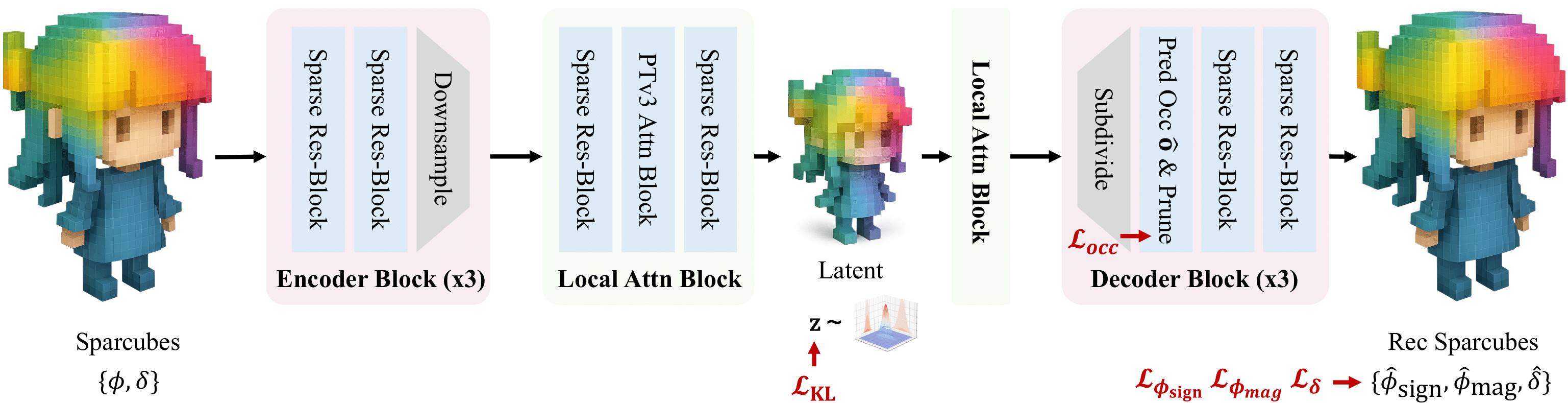
Figure: DINO feature 대신 Voxel indices 와 SDF values 를 직접 압축하는 효율적인 Sparc3D 의 Sparconv-VAE.

이러한 두 가지 상반된 관점은 3D 생성 모델의 미래에 대한 두 갈래로 나눠질 수 있다고 생각한다:

Vecset-based 모델에 VA-VAE의 아이디어를 적용하여, 의미론적으로 구조화된 latent-space 을 만들면 학습 속도와 성능을 모두 잡을 수 있을까?
아니면, 현재의 트렌드처럼 Vision Model 과의 결별을 택하고, 순수하게 3D 데이터의 공간적/위상적 특성을 고해상도로 모델링하는 데 집중하는 것이 정답일까?

이 질문에 대한 답을 찾아가는 과정이 바로 다음 세대의 3D Foundation 연구들이 집중할 방향이라고 생각한다.

마치며

이번 글에서는 3D Shape 생성을 위한 DiT 기반 모델의 내부를, 데이터 표현 방식의 차이점(Vecset vs Voxel)에 따라 비교하며 깊이 있게 분석해보았다.

이 시리즈의 다음 글에서는 본격적으로 Multi-Node, Multi-GPU 환경을 구축하고, DeepSpeed와 FSDP 같은 메모리 최적화 라이브러리의 sharding 전략을 사용하여 거대한 3D Generative Model 을 효율적으로 학습시키는 실전 전략에 대해 다뤄볼 예정이다.

원래 이 글의 후속으로 multi-node 학습을 다루려 했으나, Flow Matching 의 중요성을 깊이 있게 설명할 필요성을 느껴 (Section D 중간에 있었으나 Flow 에 대한 자세한 설명이 길어지다 못해 글의 분량을 다 잡아 먹을 것 같아...) Flow A-to-Z 를 상세하게 설명하는 별도의 글로 분리하였다: From Flow Matching to Optimal Transport: A Physics-based View of Generative Models
해당 글에서는 Normalizing Flow 의 정의에서부터 Recitified Flow 까지 자세하게 설명하고, Optimal Transport 와 연결하여 대체 왜? Recitified Flow 가 직선 경로를 채택하였는지 상세하게 설명한다.

Stay Tuned!

References

Vecset-based VAE

3D Generation w/ vecset-based VAE

Sparse-Voxel VAE (& its 3D Generation)

Hwan Heo (허환)

기타치는AI Researcher

이전 포스트

Building Large 3D Generative Models (1) - 3D Data Pre-processing

다음 포스트