[Review] Mip-NeRF: A Multiscale Representation for Anti-Aliasing Neural Radiance Fields

Hwan Heo·2022년 6월 26일

NeRF

목록 보기

4/8

NeRF 의 등장 이후 3D novel-view synthesis 분야는 NeRF's family 의 범람을 맞이했다. 하지만 Vanilla NeRF 는 real-world task 로 적용하기에는 여러가지 한계점이 있으며, (e.g, Slow convergence & inference (rendering) rate, Dataset, Background <-> Foreground... ) 그 중 한 가지는 Quantization 으로 Ray casting 을 근사하기 때문에 발생할 수 있는 Aliashing 문제이다. Mip-NeRF 의 저자들은 Ray 에서 particle 을 sampling 하는 현재의 Ray Casting 방식 대신에, CG 의 Mip-Map 기법에서 착안한 Cone-Casting-Based Mip-NeRF 를 제안한다.
ICCV2021 Oral

1. Introduction

NeRF 는 Neural Network (MLP) 의 non-linear function 에 대한 well-approximation 능력을 바탕으로, 주어진 공간 상의 특정한 particle 의 oppcaity $(\sigma)$ 와, 특정한 direction 에서 이를 바라볼 때 이 particle 의 색 (RGB) 를 예측하도록 설계된 Model 이다. (NeRF Review)

NeRF 의 정의에서 Projected Color $C(r)$ 은 다음과 같이 정의되는데,

C(r) = \int_{t_n}^{t_f} T(t) \cdot \sigma ({\rm \textbf{r}}(t)) \cdot c({\rm \textbf{r}}(t), {\rm \textbf{d}} ) \ dt \quad \text{where }T(t) = \text{exp} \bigg( - \int_{t_n}^{t}\sigma ({\rm \textbf{r}}(s)) ds \bigg )

실제 학습에서는 이를 discreatization 하는 다음과 같은 식을 통해서 NeRF 를 학습하게 된다.

C(r) = \sum_{i=1}^{N} T_i \cdot (1- \text{exp}(-\sigma_i \delta_i)) \cdot c_i, \ \quad \text{where }T_i = \text{exp} \bigg( - \sum_{j=1}^{i-1}\sigma_j \delta_j \bigg )

이러한 discreatization 에 대한 문제는, 학습 이미지 이상의 고해상도를 렌더링 할 때의 NeRF 가 aliashing 등으로 인한 artifacts 를 생성할 수 있다는 것이다. SuperSampling 등의 방식을 통해 이를 해결할 수 있겠지만, 이는 너무 느리다는 단점이 존재한다.

NeRF의 aliashing 문제를 해결하기 위해서, 저자들은 anti-aliashing 의 한 기법인 Mip-Map 에 주목한다. Mip-Map 은 어떠한 texture object 를 multi-scale 로 저장하여 geometry 에 따라 적절한 해상도의 texture 를 선택하여 표현하는 기법이다. Supersampling 등의 기법과 대비하여 이는 anti-aliashing 을 학습이 아닌 inference 단계에서 실행하게 되므로, training computational burden 을 줄일 수 있다. (Pre-Filtering)

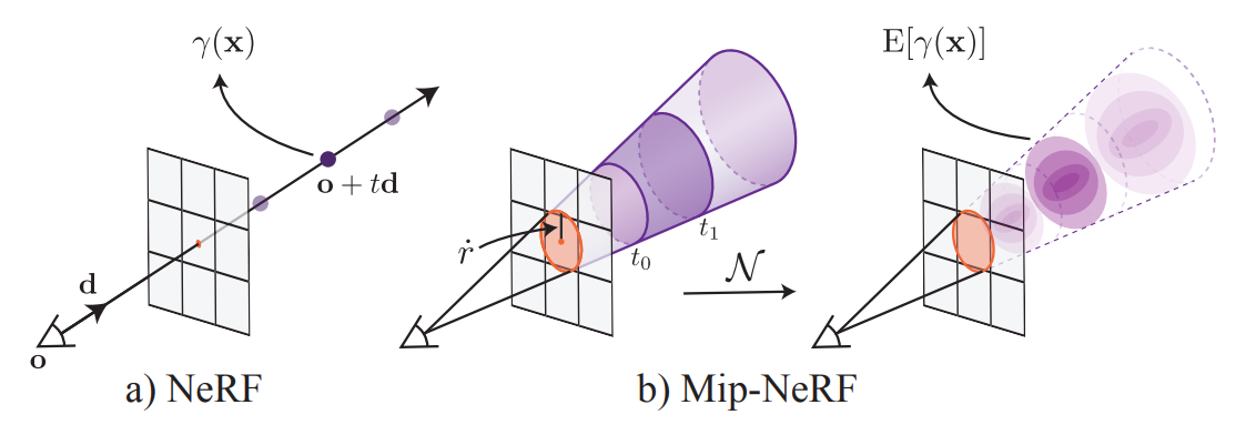
Mip-Map 에 착안하여 저자들은 pixel 이 아닌 area 의 color 를 계산하는 Mip-NeRF 를 제안한다. Mip-NeRF 는 위의 그림과 같이 a) ray 를 따라 pixel 을 렌더링하는 Ray Casting 방식이 아닌, b) pixel 과의 거리에 따른 multi-scale area 를 렌더링하는 Cone Casting 방식을 사용한다.

2. Methods

2.1. Cone Tracing and Positional Encoding

2.1.1. Cone Tracing

앞서 설명한 바와 같이 NeRF 와 대비되는 Mip-NeRF 의 가장 큰 특징은, Ray 가 아닌 Cone 을 Casting 한다는 데 있다. 즉 우리는 Cone Casting 을 위해 공간 상의 특정한 점을 Cone 의 일정 영역인 conical frustrum 으로 나타낼 수 있어야 한다.

Camera center $(\mathbf{o})$ 와 한 particel (pixel) 을 바라보는 방향 $(\mathbf{d})$ 를 생각하자.
주어진 pixel 이 나타내는 영역의 크기를 $\dot r$ 이라 할 때, (world coordinate's width scaled by $2/\sqrt 12$ ), Cone 의 중심을 지나는 직선 위의 $t$ 에 대해서 구간 $[t_0, t_1]$ 사이에 존재하는 position $\mathbf{x}$ 는 다음 정의된 $\rm F$ 의 함숫값이 1인 점들의 집합으로 정의할 수 있다.

{\rm F ({\rm \mathbf{x,o,d,}} }\dot r, t_0, t_1 ) = \mathbf{1} \left \{ { \left ( t_0 < { {\mathbf d ^ {\rm T} (\mathbf x - \mathbf o )} \over \| \mathbf d \|_2 } < t_1 \right ) \land \left ( { {\mathbf d ^ {\rm T} (\mathbf x - \mathbf o )} \over \| \mathbf d \|_2 \| \mathbf x - \mathbf o \| _2 } > {1 \over { \sqrt {1 + (\dot r / \| \mathbf d \| _2 )^2} }} \right ) } \right \}

(여기서 $\mathbf 1$ 은 indicator function 이다. velog 수식엔 mathbbm 이 안 먹어서 어쩔 수 없이 mathbf 로....)

${\rm F ({\rm \mathbf{x,o,d,}} }\dot r, t_0, t_1 )$ 의 Indicator function 안에서,

좌변: position $\mathbf x$ 를 직선에 사영했을 때 $[t_0, t_1]$ 인지
우변: position $\mathbf x$ 와 직선에 대한 cos similiarity 가 현재 scale area 에 속하는지

를 판별하게 된다.

2.1.2. Integrated Positional Encoding

Vanilla NeRF 가 고해상도로 scene reconstruction 을 진행하기 위해서는, low-dimensional input 인 $(x,y,z,\theta, \phi)$ 를 high-dimension 으로 mapping 하는 positional encoding 이 필수적이다. (Fourier Features Let Networks Learn High Frequency Functions in Low Dimensional Domains 리뷰)

이와 마찬가지로 우리는 특정한 conical frustrum 이 나타내는 영역을 positional encoding 과 같은 방법으로 high-dimension 으로 mapping 해줄 필요가 있다. i.e., Construct a featurized representation of the conical frustrum.

Ideal 한 featurized representation of conical frustrum $\gamma^*$ 은 conical frustrum 내의 모든 점에 대한 positional encoding 의 expected value 일 것이다. 즉,

\gamma^* { ({\rm \mathbf{o,d,}} }\dot r, t_0, t_1 ) = { {\int \gamma (\mathbf x) {\rm F ({\rm \mathbf{x,o,d,}} }\dot r, t_0, t_1 )d\mathbf x} \over {\int {\rm F ({\rm \mathbf{x,o,d,}} }\dot r, t_0, t_1 )d\mathbf x} }

으로 정의할 수 있다.

하지만 Continous 하게 정의된 위의 optimal $\gamma^*$ 는 computationally infeasible 하기 때문에, 이를 multivariate Gaussian 으로 근사하는 Integrated Positional Encoding (IPE) 을 제시한다.

1st Step: Characterization of Gaussian

우선 wordl coordinate $(x,y,z)$ 를 conical coordinate $\varphi(r,t,\theta) = (rt \cos \theta, rt \sin \theta, t)$ 로 나타내자 $( \theta \in [0, 2\pi ), \ t \ge 0. \ |r| \le \dot r)$ . 여기서 $(r,t,\theta)$ 는 각각,

$r$ : Area (원) 의 크기 (radius)
$t$ : Area 에 대한 Cone 의 높이 $t$
$\theta$ : Area 위의 한 점에 대한 중심과의 이루는 각

을 의미한다 (z-axis 에 중심이 있는 Cone 을 생각해보면 됨).

이를 통해 Cartessian Space $(x,y,z)$ 의 Conical Space 에서의 differential term 을 다음과 같이 유도할 수 있다.

\begin{aligned} dx\ dy\ dz &= |\text{det} (D \varphi) (r,t,\theta) | dr\ dt\ d\theta \\ & = \left\rvert \begin{matrix} t \cos \theta & t \sin \theta & 0 \\ r \cos \theta & r \sin \theta & 1 \\ -rt \sin \theta & rt \cos \theta & 0 \end{matrix} \right\rvert dr\ dt\ d\theta \\ &= (rt^2 \cos ^2 \theta + rt^2 \sin ^2 \theta ) dr\ dt\ d\theta \\ &= rt^2 \ dr\ dt\ d\theta \end{aligned}

즉 $\varphi(r,t,\theta) = rt^2$ 이며, 이를 통해 Conical frustrum 의 volume V 를 구할 수 있다.

\begin{aligned} V &= \int _0 ^{2\pi} \int _{t_0}^{t_1} \int _0 ^{\dot r} \varphi (r,t,\theta) \ dr\ dt\ d\theta \\ & = \int _0 ^{2\pi} \int _{t_0}^{t_1} \int _0 ^{\dot r} rt^2 (r,t,\theta) \ dr\ dt\ d\theta \\ &= \pi \dot r^2 { {t_1 ^3 - t_0 ^3} \over {3} } \end{aligned}

이제 우리는 Conical frustrum 에서 position $\varphi$ 에 대한 probability density function $P(r,t,\theta) = {rt^2 / V}$ 을 정의할 수 있으며, 이를 통해 $\mathbb E[t],\ \mathbb E[t^2],\ \mathbb E[x],\ \mathbb E[y]$ 을 유도할 수 있다 (cf. $r \sim \sqrt{x^2 + y^2 }$ ).

\begin{aligned} \mu _t = {3(t_1 ^4 - t_0^4) \over {4(t_1 ^3 - t_0^3 )}}, \quad \sigma_t ^2 &= {3(t_1 ^5 - t_0^5) \over {5(t_1 ^3 - t_0^3 )}} - \mu_t^2, \quad \sigma_r ^2 = \dot r ^2 \left ( { 3(t_1 ^5 - t_0^5) \over {20(t_1 ^3 - t_0^3 )} } \right ) \\ \textit{cf. } \ \mathbb E[f(t)] &= {1 \over V} \int _0 ^{2\pi} \int _{t_0}^{t_1} \int _0 ^{\dot r} f(t) \cdot P(r,t,\theta) \ dr\ dt\ d\theta \end{aligned}

$\mu_t$ : mean distance along the ray
$\sigma_t$ : variance along the ray
$\sigma_r$ : variance perpendicular to the ray

각 값들의 denominator 가 $t_1 - t_0$ 를 포함하고 있으므로, 이는 numerically unstable 한 결과를 초래할 수 있다. 따라서 저자들은 $t_\mu = (t_0 + t_1 )/2, \ t_\sigma = (t_1 - t_0 )/2$ 을 이용해 다음과 같이 reparametrization 한 값을 사용하였다.

\mu _t = t_\mu + {2t_\mu t_\sigma^2 \over {3t_\mu ^2 + t_\sigma ^2 }}, \quad \sigma_t ^2 = {t_\sigma ^2 \over 3} - {4t_\sigma^4 (12t_\mu ^2 - t_\sigma^2) \over {15(3t_\mu ^2 + t_\sigma^2 )^2}} - \mu_t^2, \quad \sigma_r ^2 = \dot r ^2 \left ( {t_\mu ^2 \over 4} + {5t_\sigma ^2 \over 12} - { 4t_\sigma ^4 \over {15(3t_\mu ^2 + t_\sigma^2 )^2} } \right )

이 때 각 Conical Frustrum 은 circular 이며 axis 에 대해 symmetric 하기 때문에 우리는 위의 $\mu_t, \sigma_t, \sigma_r$ 을 통해 Conical Space 에서의 Gaussian 을 characterize 할 수 있다.

이제 최종적으로 우리는 Conical coordinate 에서의 Gaussian 을 통해 world coordinate 의 Gaussian 을 나타낼 수 있다.

\mathbf \mu = \mathbf o + \mu_t \mathbf d , \quad \mathbf \Sigma = \sigma ^2 _t ( \mathbf d \mathbf d ^{\rm T} )+ \sigma^2 _r \left( \mathbf I - {\mathbf d \mathbf d ^{\rm T} \over \| \mathbf d \| ^2_2} \right)

2nd Step: Integrated Positional Encoding

이제 Fourier Feature Positional Encoding $\gamma (x)$ 을 matrix $\mathbf P$ 를 이용해서 나타내보자.

\gamma (\mathbf x) = \begin{bmatrix} \sin(\mathbf P \mathbf x ) \\ \cos(\mathbf P \mathbf x ) \end{bmatrix} \\ \text{where } \mathbf P = \begin{bmatrix} 1 & 0 & 0 & 2 & 0 & 0 & & 2^{L-1} & 0 &0 \\ 0 & 1 & 0 & 0 & 2 & 0 & \dots & 0 & 2^{L-1} &0 \\ 0 & 0 & 1 & 0 & 0 & 2 & & 0 & 0 &2^{L-1} \end{bmatrix} ^{\rm T}

$\text{Cov}[\mathbf Ax,\mathbf By] =\mathbf A\text{Cov}[x,y]\mathbf B^{\rm T}$ 로부터, Positional Encoding $\gamma$ 가 적용된 position $\mathbf x$ 에 대한 Gaussian 은 다음과 같다.

\mathbf \mu_\gamma = \mathbf P\mathbf \mu, \quad \mathbf \Sigma _\gamma = \mathbf P \mathbf \Sigma \mathbf P^{\rm T}

이제 삼각함수에 대한 gaussian 의 expectation

\begin{aligned} & \mathbb E_{x \sim \mathcal N(\mu, \sigma^2)} [ \sin x] = \sin (\mu) \exp (- (1/2)\sigma^2), \\ & \mathbb E_{x \sim \mathcal N(\mu, \sigma^2)} [ \cos x] = \cos (\mu) \exp (- (1/2)\sigma^2) \end{aligned}

을 이용하여 IPE feature $\gamma(\mathbf \mu,\mathbf \Sigma)$ 는 최종적으로 다음과 같이 정의된다.

\begin{aligned} \gamma(\mathbf \mu,\mathbf \Sigma) &= \mathbb E_{\mathbf x \sim \mathcal N(\mu, \sigma^2)} [ \gamma( x)] \\ &= \begin{bmatrix} \sin (\mathbf \mu_\gamma) \circ \exp (- (1/2)\text{diag}(\mathbf \Sigma_\gamma)) \\ \cos (\mathbf \mu_\gamma) \circ \exp (- (1/2)\text{diag}(\mathbf \Sigma_\gamma)) \end{bmatrix}. \end{aligned}

이 때 $\mathbf \Sigma_\gamma$ 을 직접적으로 계산하는 대신 (prohibitively expensive to compute), $\text{diag}(\mathbf \Sigma_\gamma)$ 을 계산하여 이용했다고 한다.

\text{diag}(\mathbf \Sigma_\gamma) = \left [\text{diag}(\mathbf \Sigma), 4\text{diag}(\mathbf \Sigma), \dots, 4^{L-1}\text{diag}(\mathbf \Sigma) \right ]^{\rm T} \\ \text{where } \mathbf \Sigma = \sigma ^2 _t ( \mathbf d \circ \mathbf d )+ \sigma^2 _r \left( \mathbf I - {\mathbf d \circ \mathbf d \over \| \mathbf d \| ^2_2} \right)

Visualization of IPE

아래 두 그림에서 PE 와 IPE 를 시각적으로 비교할 수 있다.

IPE 가 wider range 를 나타낼수록 high-frequency 를 softly remove 하며 다시 말해 일종의 smooth 한 Low-pass Filter 처럼 작동하는 것을 알 수 있다. Low-pass Filter 는 대표적인 Anti-alsiashing 의 한 방법으로, IPE 가 자연스럽게 Anti-alsiashing 을 야기할 것임을 알 수 있다.

또한 저자들은 IPE 의 장점으로 hyperparameter $L$ 튜닝에 robust 하다고 주장한다. Fourier Features Let Networks Learn High Frequency Functions in Low Dimensional Domains 에 따르면, $L$ 은 일종의 cut off frequency 를 결정하는 hyperparameter 로 적용된다.

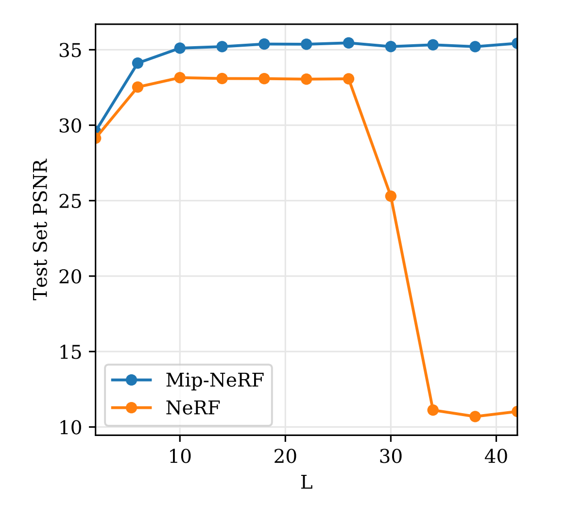
반면 Gaussian 으로 근사되는 IPE 의 경우에는 area 의 scale 에 따라 이러한 truncation 이 soft 하게 적용되기 때문에 $L$ -invariant 한 결과를 얻는다고 한다. 아래의 실험에서 이를 확인할 수 있는데, PE 의 경우 일정 이상의 $L$ 에 대해서 심각한 overfitting 이 일어나는반면, IPE 에서는 그렇지 않은 것을 알 수 있다.

2.2. Architecutre

2.2.1. Training Objective & Hierarchical Strategy

Cone Tracing 을 위시한 IPE 를 input 으로 사용하는 것 외의 Mip-NeRF 와 NeRF 의 차이점은 많지 않지만, 한 가지 주요한 차이점은 NeRF 의 hierarchical sampling 을 단일 Network 를 통해 구현할 수 있다는 데 있다.

Vanilla NeRF 에서의 coarse network 와 fine network 는 quantization rate 가 다르기 때문에 각각 low resolution <-> high resolution 으로 학습된 network 라고 생각할 수 있다. 이는 Vanilla NeRF 는 multi-scale ability 가 없기 때문이다.

이에 반면 Mip-NeRF 는 cone tracing 으로 multi-scale 을 나타낼 수 있으며, single Mip-NeRF network 로 hierarchical sampling 을 진행할 수 있다. 즉, parameters of a single Mip-NeRF $\Theta$ 를 학습하는 Training Objective 는 다음과 같다.

\min_{\Theta} \sum_{r \in \mathcal R} \bigg ( \lambda \big \| C^*(r) - \textbf{C}(r; \Theta, t^c) \big \|_2 ^2 + \big \| C^*(r) - \textbf{C}(r; \Theta, t^f) \big \|_2 ^2 \bigg )

여기서 $t^c, t^f$ 는 각각 Vanilla NeRF 처럼 stratified sampling 과 이를 통해 구한 weight 로 inverse sampling 을 통한 coarse, fine sampling 이다.

$t^f$ 의 sampling 전에 weight 에 다음과 같은 filter 를 적용하였다고 한다.

w'_k = {1 \over 2} (\max (w_{k-1}, w_k ) + \max(w_k, w_{k+1} ) ) + \alpha

식을 보면 일종의 moving average 처럼 작용함을 알 수 있는데, 이를 통해 wide & smooth upper 한 weight 를 생성하여 사용하였다고 한다.

이는 stratified sampling 의 결과에 일종의 blur filter 를 적용한 것과 같은데, 즉 이 자체로 anti-aliashing 의 효과가 있다. Experiments 에서는 weight modification 에 대한 ablation 이 존재하지 않는데 이에 대한 ablation 도 있었으면 좋았을 것 같다.

2.2.2. Model Details

이 부분은 supplementary material 에 재구현을 위해서 자세하게 작성되어 있다.

1) Identity Concatenation

Original NeRF에서의 positional encoding 은 다음과 같이 Identity Concatenation 을 사용한다.

\mathbf x = \mathbf x + \gamma(\mathbf x)

Mip-NeRF 에서는 이러한 setting 이 performance 향상에 도움을 주지 않아서 IPE 그대로만 사용했다고 한다.

2) Activation Functions

Original NeRF 에서 사용되는 두 activation funcions 1) ReLU, 2) Sigmoid 를 각가 다음으로 대체하였다.

Relu $\rightarrow \log(1+\exp(x-1))$ , i.e. softplus
Sigmoid $\rightarrow (1+2\epsilon)/(1+\exp(-x))-\epsilon$ , i.e. widened sigmoid

3. Experiments

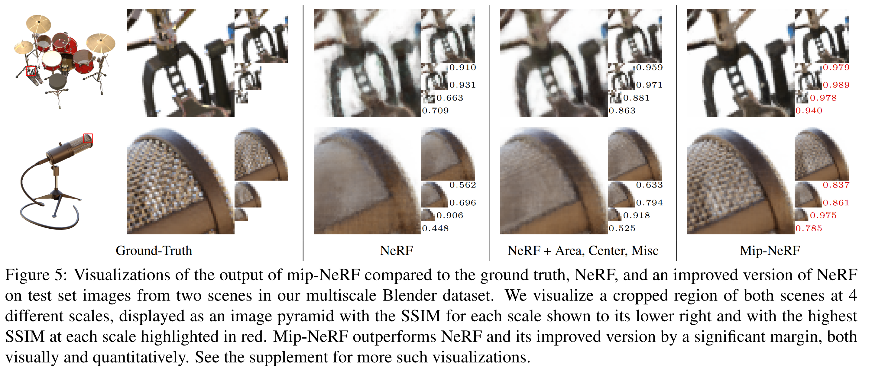
위의 Qualitative Results 는 left: NeRF, right: Mip-NeRF 를 나타낸 것이다. NeRF 가 multi-scale 에서의 결과가 망가지는데 반면에, Mip-NeRF 는 그렇지 않은 것을 시각적으로 확인할 수 있다.

Figure 를 통해서 Mip-NeRF 의 multi-scale 에서의 능력을 잘 보여주는데, 이를 마치 mip-map 처럼 visualize 하여 약간의 웃음 포인트였다.

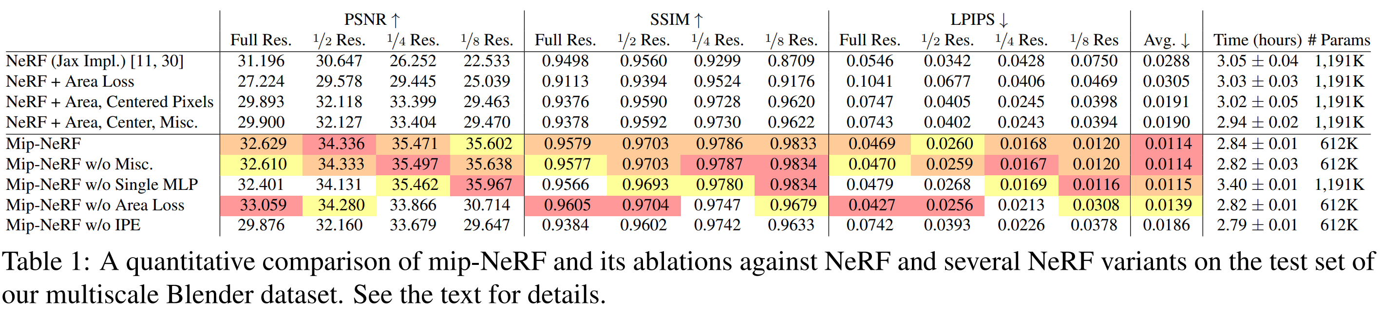
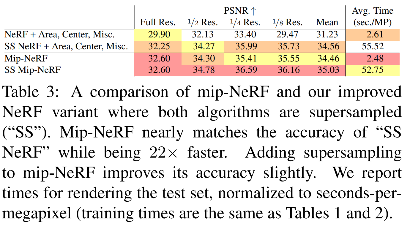
Qualitative results 외에도 quantitative results 로 Mip-NeRF 의 multi-scale performance 가 Table1, Table3 에 잘 나타나 있다. 전체적으로 Vanilla NeRF 과 비교해 월등한 결과를 보이면서도 Supersampling 기법을 사용하는 NeRF 보다 효율적으로 학습될 수 있음을 보여주고 있다.