출처: 코리 웨이드.(2022). XGBoost와 사이킷런을 활용한 그레이디언트 부스팅. 서울:한빛미디어
Data Encoding
Data Loading
import pandas as pd
import warnings

pd.options.display.max_columns = None # pandas 출력 column 개수 제한 해제
warnings.filterwarnings('ignore')

df = pd.read_csv('student-por.csv', sep=';') # ';' 구분자
df.head(2)
Missing Value
x = df.isnull().sum()
x[x!=0] # 결측치가 존재하는 column만 선택 (sex, age, guardian)- sex, age, guardian column에 1개의 데이터씩 결측치가 존재
- 결측치 데이터 확인
df[df.isna().any(axis=1)] # 결측치 위치 확인
- 결측치가 존재하는 column type 확인
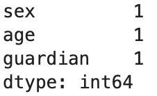
missing_cols = x[x!=0].index
df.dtypes[missing_cols]  # 수치형(age), 범주형(sex, guardian)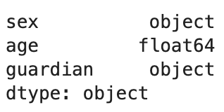
- 결측치 처리
-
수치형 변수: 특정값으로 대체 (ex. -999.0)
-
범주형 변수:
- 최빈값으로 대체
- 누락된 값이 많을 경우, 최빈값으로 결측치를 채울 때 분포가 왜곡될 수 있음
- unknown과 같이 결측치를 특정하는 값으로 대체
- 최빈값으로 대체
-
Column별 대체 값
- sex (F: 382, M: 266) → F
- guardian (mother:454, father: 153, other:41) → motherdf['age'] = df['age'].fillna(-999.0) df['sex'] = df['sex'].fillna(df['sex'].mode()) df['guardian'] = df['guardian'].fillna(df['guardian'].mode())
-
One-Hot Encoding
pd.get_dummies()- 범주형 특성을 0(값 없음), 1(값 있음)의 수치형으로 변환
- 단점
- 계산 비용이 많이 들 수 있음
- scikit-learn 파이프라인에 통합되지 않음
- scikit-learn
OneHotEncoder클래스-
모든 범주형 특성을 0, 1로 encoding
-
희소 행렬을 사용하기 때문에 계산 비용이 높지 않음
- 희소 행렬은 0이 아닌 값만 저장하여 공간을 절약함
-
scikit-learn의 파이프라인과 사용할 수 있음
- scikit-learn 0.20 version부터 가능
- 이전 버전 OneHotEncoder는 수치형 특성만 받았기 때문에,
LabelEncoder로 범주형 특성을 수치형으로 변환 후 사용해야됐음from sklearn.preprocessing import OneHotEncoder # category column만 추출 # categorical_columns = df.columns[df.dtypes==object].tolist() # 책에 있는 방법 categorical_columns = df.select_dtypes(include=['object']).columns.tolist() # 다양한 데이터 타입을 뽑을 수 있음 ohe = OneHotEncoder() hot = ohe.fit_transform(df[categorical_columns]) # 희소 행렬로 encoding (1만 저장) hot_df = pd.DataFrame(hot.toarray()) # 희소 행렬을 밀집 행렬로 변환 (0, 1 둘다 보여줌) hot_df.head(2) -
위 코드에서
hot변수 확인

hot_df.sum().sum() == 11033 # True -> 1만 저장하는 것을 알 수 있음
print(hot)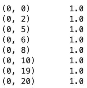
-
수치형 특성과 One-hot Encoding된 특성 합치기
- 수치형 특성 추출
cold_df = df.select_dtypes(exclude=["object"]) - 방법 1
-
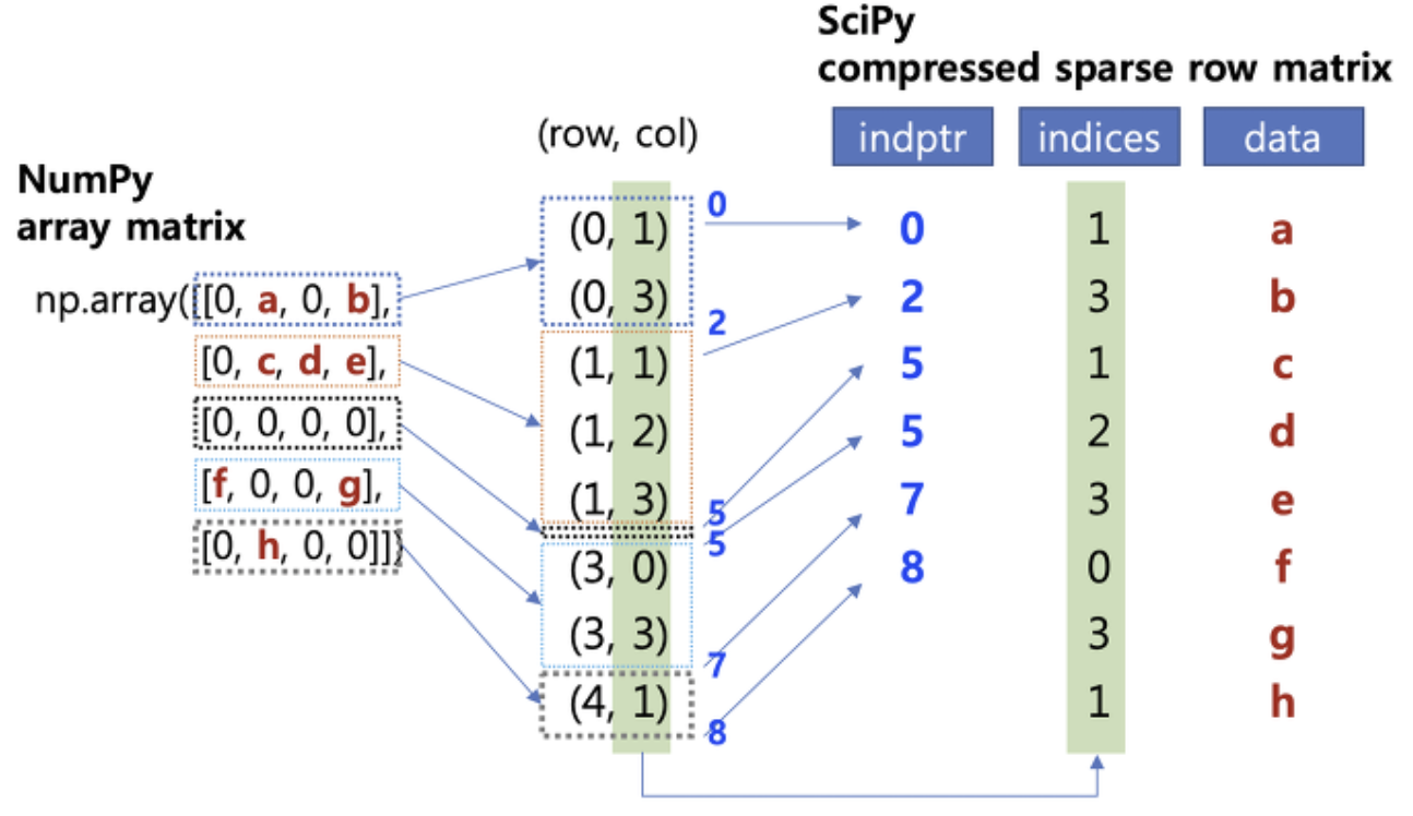
scipy.sparse 모듈의 csr_matrix() 함수를 사용
- Compressed Sparse Row(CSR): 가로의 순서대로 재정렬하는 방법으로 행에 관여하여 정리 압축
%time
from scipy.sparse import csr_matrix
cold = csr_matrix(cold_df) # 희소 행렬로 변환

from scipy.sparse import hstack
final_sparse_matrix = hstack((hot, cold)) # 열 기준 추가 (수평 연결)

final_df = pd.DataFrame(final_sparse_matrix.toarray()) # 밀집 행렬로 변환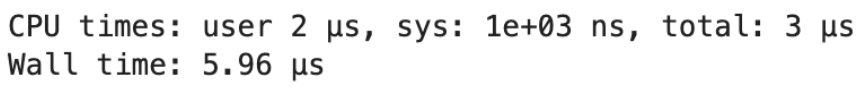
-
- 방법 2
%time
hot_df = pd.DataFrame(hot.toarray()) # 희소 행렬을 밀집 행렬로 변환 (0, 1 둘다 보여줌)
final_df = pd.concat([hot_df, cold_df], axis=1) # 열 기준 추가 (수평 연결)
final_df.columns = list(range(len(final_df.columns))) # column명 변경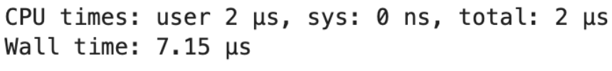
→ 방법 1의 속도가 미세하게 빠름 (데이터가 클수록 차이가 클 것으로 예상됨)
사용자 정의 scikit-learn 변환기
- 변환기 → 작업의 반복을 줄여서 시간을 아낄 수 있음!
관련 class 종류
StandardScaler: 데이터 표준화Normalizer: 데이터 정규화SimpleImputer: 누락된 값 대체- strategy: 누락된 값을 처리하는 방식 지정 (default: mean)
- mean: 평균
- median: 중앙값
- most_frequent: 최빈값
- constant: 임의값 (fill_value에 대체할 값을 전달해야됨)
- strategy: 누락된 값을 처리하는 방식 지정 (default: mean)
TransformerMixin클래스 상속 → 사용자화fit(): 변환에 필요한 통계값 추출transform(): 통계값을 적용하여 데이터를 변환- 결측치 대체 변환기 예시 code
from sklearn.base import TransformerMixin

class NullValueImputer(TransformerMixin):

    def __init__(self):
        None

    def fit(self, X, y=None):
        return self

    def transform(self, X, y=None):
        for column in X.columns.tolist():
            if column in X.columns[X.dtypes==object].tolist():
                X[column] = X[column].fillna(X[column].mode()) # 최빈값
            else:
                X[column]=X[column].fillna(-999.0) # 임의값

        return X

test = NullValueImputer().fit_transform(df)
ColumnTransformer- 입력 데이터의 column마다 다른 변환기를 적용 가능
- 적용할 변환기는
(이름, 변환기 객체, column 인덱스 or 이름)과 같은 튜플의 리스트로 지정 - remainder (default: drop)
-
passthrough: 결과 배열에 그대로 포함
-
drop: 사용하지 않는 특성은 삭제
from sklearn.compose import ColumnTransformer
from sklearn.impute import SimpleImputer

# SimpleImputer 객체 초기화
mode_imputer = SimpleImputer(strategy='most_frequent')
const_imputer = SimpleImputer(strategy='constant', fill_value=-999.0)

# 범주형/수치형 column 추출
categorical_columns = df.columns[df.dtypes==object].tolist()
numeric_columns = df.columns[df.dtypes!=object].tolist()

# ColumnTransformer 객체 초기화
ct = ColumnTransformer([('str', mode_imputer, categorical_columns),
                        ('num', const_imputer, numeric_columns)])

# column별 변환기 적용
new_df = pd.DataFrame(ct.fit_transform(df),
                      columns=categorical_columns+numeric_columns)

# 원본 데이터프레임과 column 순서 동일하게 setting
new_df = new_df[df.columns]
-
- One-hot 인코딩 적용 (방법 1 - TransformerMixin)
class SparseMatrix(TransformerMixin): def __init__(self): self.ohe = OneHotEncoder() # 객체 초기화 def fit(self, X, y=None): self.categorical_columns= X.columns[X.dtypes==object].tolist() self.ohe.fit(X[self.categorical_columns]) # 객체 훈련 return self def transform(self, X, y=None): hot = self.ohe.transform(X[self.categorical_columns]) # 범주형 변수 one-hot 인코딩 변환 (희소행렬) cold_df = X.select_dtypes(exclude=["object"]) # 수치형 변수 추출 cold = csr_matrix(cold_df) # 수치형 변수 희소행렬로 변환 final_sparse_matrix = hstack((hot, cold)) # 수평 연결 return final_sparse_matrix sm = SparseMatrix().fit_transform(nvi) # 희소 행렬 sm_df = pd.DataFrame(sm.toarray()) # 밀집 행렬 - One-hot 인코딩 적용 (방법 2 - ColumnTransformer)
ct2 = ColumnTransformer([('ohe', OneHotEncoder(), categorical_columns)],
                       remainder='passthrough') # 범주형 변수만 one-hot encoding 적용

ct2.fit(new_df) # 훈련
oh_columns = ct2.named_transformers_['ohe'].get_feature_names_out() # one-hot 인코딩된 특성 이름 추출

new_df2 = pd.DataFrame(ct2.transform(new_df),
                       columns=np.append(oh_columns, numeric_columns))
전처리 파이프라인
- 테스트 세트는 별도로 분리하는 것이 중요
from sklearn.model_selection import train_test_split df = pd.read_csv('student-por.csv', sep=';') y = df.iloc[:, -1] X = df.iloc[:, :-3] # 마지막 2,3번째 column은 종속 변수와 관련있어서 제외 X_train, X_test, y_train, y_test = train_test_split(X, y, random_state=2) - 결측치 처리, 희소 행렬 변환 pipeline 만들기
from sklearn.pipeline import Pipeline

data_pipeline = Pipeline([('null_imputer', NullValueImputer()),
                          ('sparse', SparseMatrix())])

X_train_transformed = data_pipeline.fit_transform(X_train).toarray()
Modeling
Hyper-parameter tuning
# 데이터 분할
X_train_2, X_test_2, y_train_2, y_test_2 = train_test_split(X_train_transformed, y_train, random_state=2)

# grid 탐색
def grid_search(params, reg=XGBRegressor(missing=-999.0)):
    grid_reg = GridSearchCV(reg, params,
                            scoring='neg_mean_squared_error', cv=kfold)
    grid_reg.fit(X_train_transformed, y_train)
    best_params = grid_reg.best_params_
    print("최상의 매개변수:", best_params)
    best_score = np.sqrt(-grid_reg.best_score_)
print("최상의 점수:", best_score)-
최적 트리 개수 파악 →
2.9043888114810597# 최상의 매개변수: {'n_estimators': 30} grid_search(params={'n_estimators':[30, 34, 50, 100, 200, 300, 500, 1000]}) -
max_depth 설정 →
2.6624068530083567# 최상의 매개변수: {'max_depth': 1, 'n_estimators': 30} grid_search(params={'max_depth':[1, 2, 3, 4, 6, 7, 8], 'n_estimators':[30]}) -
min_child_weight 파악 (max_depth 범위는 1~2로 축소) →
2.6586291790662853# 최상의 매개변수: {'max_depth': 1, 'min_child_weight': 9, 'n_estimators': 30} grid_search(params={'max_depth':[1, 2], 'min_child_weight':[1, 2, 3, 4, 5, 6, 7, 8, 9, 10], 'n_estimators':[30]}) -
subsample 0.5~0.9 탐색, n_estimator 케이스 추가 →
2.655334578520487# 최상의 매개변수: {'max_depth': 1, 'min_child_weight': 8, 'n_estimators': 50, 'subsample': 0.8} grid_search(params={'max_depth':[1], 'min_child_weight':[8, 9, 10], 'subsample':[0.5, 0.6, 0.7, 0.8, 0.9], 'n_estimators':[34, 50]}) -
colsample_bytree 탐색, subsample 범위 축소 →
2.650728722526981# 최상의 매개변수: {'colsample_bytree': 1, 'max_depth': 1, 'min_child_weight': 9, 'n_estimators': 40, 'subsample': 0.8} grid_search(params={'max_depth':[1], 'min_child_weight':[8, 9, 10], 'subsample':[0.8, 0.9, 1], 'colsample_bytree':[0.5, 0.6, 0.7, 0.8, 0.9, 1], 'n_estimators':[40, 50, 60]}) -
colsample_bynode, colsample_bylevel 추가 →
2.627934932234306# 최상의 매개변수: {'colsample_bylevel': 0.7, 'colsample_bynode': 0.6, 'colsample_bytree': 1.0, 'max_depth': 1, 'min_child_weight': 10, 'n_estimators': 40, 'subsample': 0.8} grid_search(params={'max_depth':[1], 'min_child_weight':[8, 9, 10], 'subsample':[0.8], 'colsample_bytree':[1.0], 'colsample_bylevel':[0.6, 0.7, 0.8, 0.9, 1], 'colsample_bynode':[0.6, 0.7, 0.8, 0.9, 1], 'n_estimators':[40]}) -
최고의 하이퍼파라미터 결과로 모델 재생성
model = XGBRegressor(max_depth=1,
                     min_child_weight=10,
                     subsample=0.8,
                     colsample_bytree=1.0,
                     colsample_bylevel=0.7,
                     colsample_bynode=0.6,
                     n_estimators=40,
                     missing=-999.0)
Model Test
- 모델 성능 평가
X_test_transformed = data_pipeline.fit_transform(X_test).toarray() model.fit(X_train_transformed, y_train) # 학습 y_pred = model.predict(X_test_transformed) # 예측 rmse = MSE(y_pred, y_test)**0.5 # 평가 -> 2.816873379911829 - 모델의 과대적합을 방지하기 위해 Hyper-parameter 조정
-
ex. min_child_weight를 높이고, subsample을 낮추기
-
테스트 점수를 높이기 위해 하이퍼파라미터 튜닝 과정을 반복하면 안됨
-
테스트 점수를 확인 후, 약간의 조정만 가능
model = XGBRegressor(max_depth=1,
                     min_child_weight=13,
                     subsample=0.6,
                     colsample_bytree=1.0,
                     colsample_bylevel=0.7,
                     colsample_bynode=0.6,
                     n_estimators=40,
                     missing=-999.0)

model.fit(X_train_transformed, y_train)
y_pred = model.predict(X_test_transformed)
rmse = MSE(y_pred, y_test)**0.5 # 2.809052153147433
-
ML Pipeline
- 누락 값 처리 + 희소 행렬 + 모델
full_pipeline = Pipeline([('null_imputer', NullValueImputer()),
                          ('sparse', SparseMatrix()),
                          ('xgb', XGBRegressor(max_depth=1,
                                               min_child_weight=13,
                                               subsample=0.6,
                                               colsample_bytree=1.0,
                                               colsample_bylevel=0.7,
                                               colsample_bynode=0.6,
                                               n_estimators=40,
                                               missing=-999.0))])
new_data = X_test # 일반화 검증
full_pipeline.fit(X, y) # 학습
full_pipeline.predict(new_data) # 예측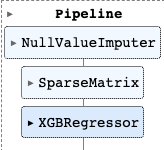
-
모델 직렬화
- 직렬화(serialization) : 파이썬 객체를 일정한 규칙(protocol)에 따라 효율적으로 저장하고 전송할 때, 데이터를 줄로 세워 저장하는 것
- 모델 저장 → pickle, json, joblib 사용 가능
model.save_model('final_xgboost_model.json') - pipeline 객체 저장 → pickle, joblib 사용
- pickle
import pickle # 객체 저장 with open('full_pipeline.pickle', 'wb') as f: pickle.dump(full_pipeline, f) # 객체 읽기 with open('full_pipeline.pickle', 'rb') as f: load_pipeline = pickle.load(f) - joblib
import joblib

joblib.dump(full_pipeline, 'full_pipeline.joblib') # 객체 저장

load_pipeline = joblib.load('full_pipeline.joblib') # 객체 읽기
- pickle
-
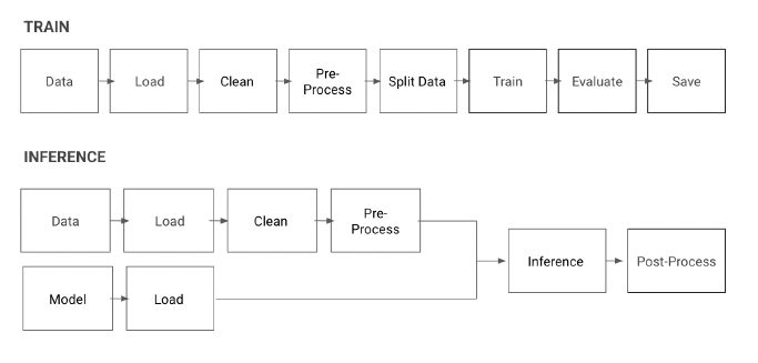
ML 파이프라인 적용 예시 (2 track)
Reference