[KDT_AISEC] 7주차 - openCV(2)

openCV

---

밝기와 대비

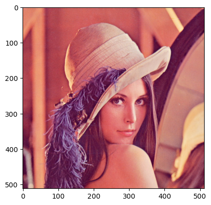
img = cv.imread('../samples/lena.jpg')
img_r = cv.cvtColor(img, cv.COLOR_BGR2RGB)
plt.imshow(img_r)

레나라는 이미지는 영상 처리 알고리즘과 관련된 작업에서 굉장히 유명한 이미지이다.

1996년 1월판 IEEE Transactions on Image Processing의 편집장이던 David C. Munson은 레나 사진을 영상처리에 널리 사용하는 이유에 대해 다음과 같이 밝혔다.

먼저, 레나 이미지는 세밀함과 평면, 그림자, 그리고 질감이 적절하게 조화되어 있어서 다양한 이미지 처리 알고리즘을 처리하는 데 좋다. 이 이미지는 정말 좋은 시험용 이미지이다. 둘째로, 레나 이미지는 매력적인 여성의 사진이다. 그러므로 이미지 처리 연구 분야 종사자들이 매력적이라고 느끼는 이미지에 끌리는 것은 대다수가 남자이기 때문에, 별로 놀라울 게 없다.

출처: 위키백과

우선 밝기와 대비의 차이를 보다 극명하게 보기 위해 이미지를 그레이 스케일로 바꿔주었다.

img = cv.cvtColor(img, cv.COLOR_BGR2GRAY)
plt.imshow(img, cmap='gray')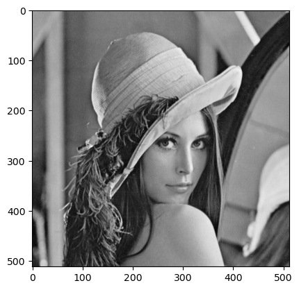

이제 이미지의 픽셀값들에 단순 수치 더하기 빼기를 진행해보자.

img1 = img - 100
plt.imshow(img1, cmap='gray')
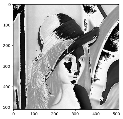
img2 = img + 100
plt.imshow(img2, cmap='gray')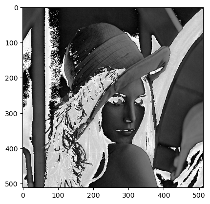

다시, openCV에서 제공하는 cv.add함수를 이용해보자.

img3 = cv.add(img, 100)
plt.imshow(img3, cmap='gray')
img3 = cv.add(img, -100)
plt.imshow(img3, cmap='gray')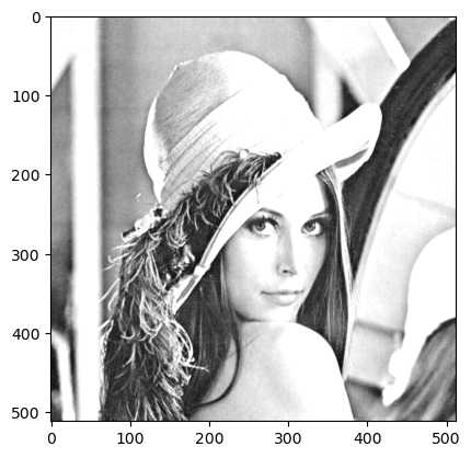

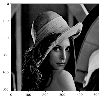
단순 더하기 빼기와는 다르게 이미지 자체가 살아있으면서 조절되는것을 볼 수 있다.

img = cv.imread('../samples/lena.jpg', cv.IMREAD_GRAYSCALE)

def on_brightness(pos, src):
    dst = cv.add(src, pos)
    return dst

cv.namedWindow('image')
cv.createTrackbar('brightness', 'image', 0, 255, lambda x: x)

while cv.waitKey(1) != 27:
    bright = cv.getTrackbarPos('brightness', 'image')
    
    img_br = on_brightness(bright, img)
    cv.imshow('image', img_br)
    
cv.destroyAllWindows()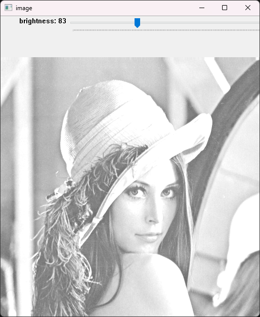

위는 트랙바를 이용해 밝기를 조절하는 프로그램이다.

def on_contrast(pos, src):
    pos -= 10
    dst = src + (src - 128) * pos
    return dst

cv.namedWindow('image')
cv.createTrackbar('contrast', 'image', 0, 20, lambda x: x)

while cv.waitKey(1) != 27:
    bright = cv.getTrackbarPos('contrast', 'image')
    
    img_br = on_contrast(bright, img)
    cv.imshow('image', img_br)
    
cv.destroyAllWindows()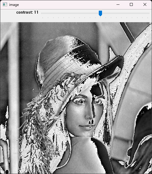

같은 방법으로 대비를 조절하는 프로그램도 작성해보았다.

변환

이미지 변환에 대해서 살펴보자.

# 이미지 크기 조정

fig = plt.figure(figsize=(10, 10))
ax1 = fig.add_subplot(1, 2, 1)
ax2 = fig.add_subplot(1, 2, 2)

img = cv.imread('../samples/messi5.jpg')

res1 = cv.resize(img, None, fx=2, fy=2, interpolation=cv.INTER_CUBIC)
print(img.shape, res1.shape)

h, w = img.shape[:2]
res2 = cv.resize(img, (2*w, 2*h), interpolation=cv.INTER_CUBIC)
print(res2.shape)

ax1.imshow(img)
ax2.imshow(res1)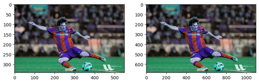

언뜻 보면 별 차이가 없어보이지만 사실은 오른쪽의 메시가 사이즈를 두배로 늘린 메시이다.

# 이미지 위치 변경

fig = plt.figure(figsize=(10, 10))
ax1 = fig.add_subplot(1, 2, 1)
ax2 = fig.add_subplot(1, 2, 2)

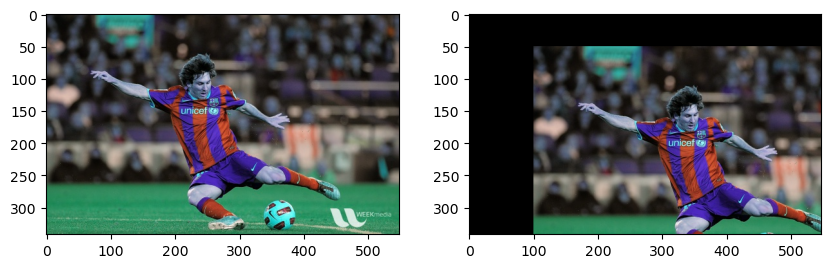
img = cv.imread('../samples/messi5.jpg')

r, c = img.shape[:2]
m = np.float32([[1, 0, 100], [0, 1, 50]])
dst = cv.warpAffine(img, m, (c, r))

ax1.imshow(img)
ax2.imshow(dst)

warpAffine함수를 이용해서 이미지의 위치를 조정할 수 있다.

# 이미지 회전

fig = plt.figure(figsize=(10, 10))
ax1 = fig.add_subplot(1, 2, 1)
ax2 = fig.add_subplot(1, 2, 2)

img = cv.imread('../samples/messi5.jpg')

r, c = img.shape[:2]
m = cv.getRotationMatrix2D(((c-1)/2.0, (r-1)/2.0), 90, 1)
dst = cv.warpAffine(img, m, (c, r))

ax1.imshow(img)
ax2.imshow(dst)

getRotationMatrix2D함수를 이용하면 이미지를 회전시킬 수 있다.

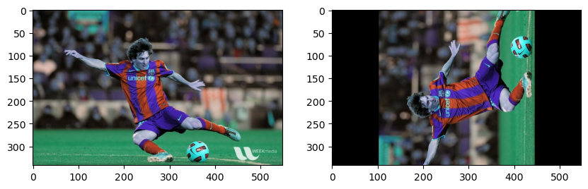
각도를 정하지 않고 반전시키는 경우에는 cv.flip함수를 이용하면 된다.

# 이미지 회전2

fig = plt.figure(figsize=(10, 10))
ax1 = fig.add_subplot(2, 2, 1)
ax2 = fig.add_subplot(2, 2, 2)
ax3 = fig.add_subplot(2, 2, 3)
ax4 = fig.add_subplot(2, 2, 4)

img = cv.imread('../samples/messi5.jpg')

r, c = img.shape[:2]

ax1.imshow(img)
ax2.imshow(cv.flip(img, -1))
ax3.imshow(cv.flip(img, 0))
ax4.imshow(cv.flip(img, 1))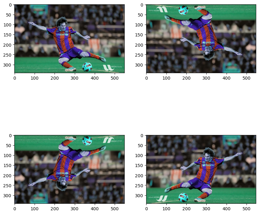

다음은 이미지 어파인 변환인데, 좌표를 지정해서 변환시키면 마치 사선으로 보는듯하게 변환시키는것도 가능하다. 이게 가능하다는것은 애초에 사선으로 되어있는 이미지를 정방향으로 보이게끔 변환할 수 있다는것을 뜻한다.

# 이미지 affine 변환

fig = plt.figure(figsize=(10, 10))
ax1 = fig.add_subplot(1, 2, 1)
ax2 = fig.add_subplot(1, 2, 2)


img = cv.imread('../samples/chessboard.png')

r, c = img.shape[:2]

pts1 = np.float32([[50, 50], [200, 50], [50, 200]])
pts2 = np.float32([[10, 100], [200, 50], [100, 250]])

m = cv.getAffineTransform(pts1, pts2)
dst = cv.warpAffine(img, m, (c, r))

ax1.imshow(img)
ax2.imshow(dst)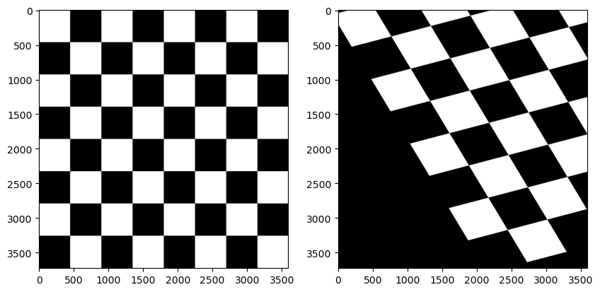

다음은 이미지 투시 변환이다. 투시 변환은 이미지 내에 존재하는 객체의 꼭짓점등을 이용하여 변환시키는 것이다.

# 이미지 투시 변환

fig = plt.figure(figsize=(10, 10))
ax1 = fig.add_subplot(1, 2, 1)
ax2 = fig.add_subplot(1, 2, 2)


img = cv.imread('../samples/sudoku.png')

r, c = img.shape[:2]

pts1 = np.float32([[70, 85], [495, 68], [30, 520], [520, 520]])
pts2 = np.float32([[0, 0], [300, 0], [0, 300], [300, 300]])

m = cv.getPerspectiveTransform(pts1, pts2)
dst = cv.warpPerspective(img, m, (300, 300))

ax1.imshow(img)
ax2.imshow(dst)

# 이미지 투시 변환

fig = plt.figure(figsize=(10, 10))
ax1 = fig.add_subplot(1, 2, 1)
ax2 = fig.add_subplot(1, 2, 2)


img = cv.imread('../samples/left04.jpg')

r, c = img.shape[:2]

pts1 = np.float32([[160, 85], [550, 50], [150, 380], [570, 400]])
pts2 = np.float32([[0, 0], [400, 0], [0, 400], [400, 400]])

m = cv.getPerspectiveTransform(pts1, pts2)
dst = cv.warpPerspective(img, m, (400, 400))

ax1.imshow(img)
ax2.imshow(dst)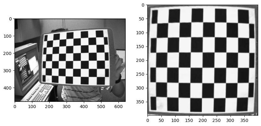

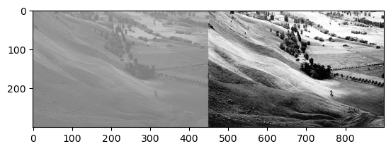
히스토그램 평탄화

이미지 히스토그램이란 어떤 이미지에서 밝은 픽셀과 어두운 픽셀의 분포를 히스토그램으로 나타낸 것이다.
이러한 이미지의 히스토그램을 평탄화시켜주면 픽셀의 분포가 치우쳐져있다가 고루 분포되기 때문에 전체적으로 조금 더 잘 보이게 된다.

fig = plt.figure(figsize=(10, 10))
ax1 = fig.add_subplot(1, 2, 1)
ax2 = fig.add_subplot(1, 2, 2)

img = cv.imread('../samples/lena.jpg',0)

ax2.hist(img.ravel(),256,[0,256])
ax1.imshow(img, cmap='gray')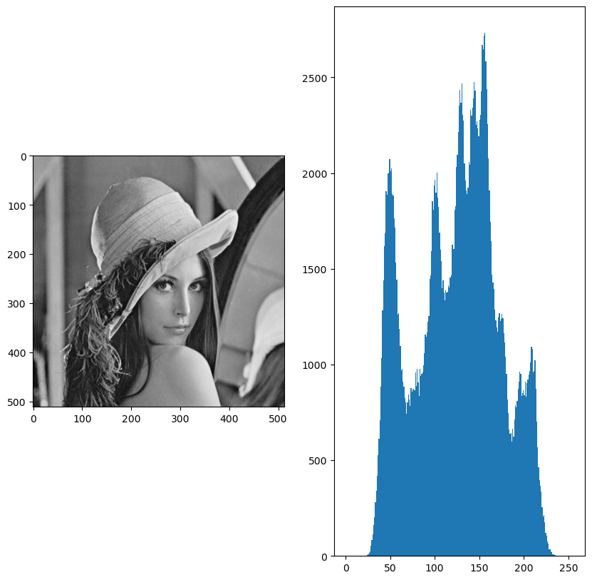

img = cv.imread('../samples/hawkes.bmp',0)
equ = cv.equalizeHist(img)
res = np.hstack((img,equ)) #stacking images side-by-side
plt.imshow(res, cmap='gray')