Logistic Classification

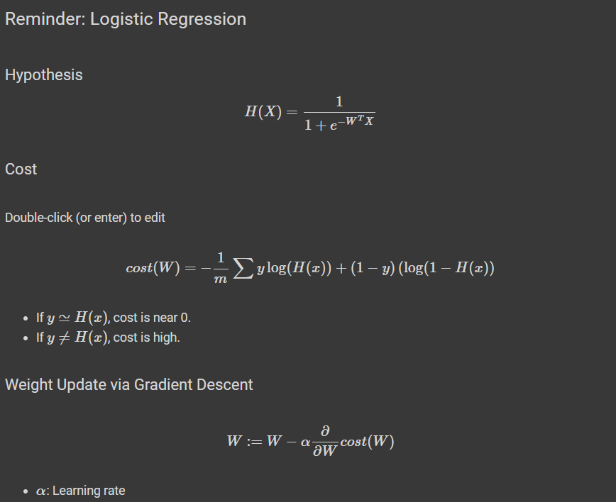
가설 설정과 활성화 함수를 위와 같이 설정을 한다면 Gradient Descent를 구할 수 있게 됩니다.

기계학습(Machine Learning) , 인공지능(AI), 딥러닝(Deep Learning)의 모든 프로세스들은
데이터 로드 -> 모델 학습 -> 데이터 평가 or 결과 예측 으로 이루어 져있습니다. 차례대로 학습 과정을 진행해보겠습니다.

데이터 로드

# pytorch
import torch
# 최적화 알고리즘 : SGD 
import torch.optim as optim


# For reproducibility
torch.manual_seed(1)

# 임의 데이터 생성
x_data = [[1, 2], [2, 3], [3, 1], [4, 3], [5, 3], [6, 2]]
y_data = [[0], [0], [0], [1], [1], [1]]


x_train = torch.FloatTensor(x_data)
y_train = torch.FloatTensor(y_data)

print(x_data)
print(x_train)

print(x_train.shape)
print(y_train.shape)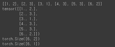

최적화 알고리즘인 SGD를 사용하기 위해 optim이라는 모듈을 import 시키고 랜덤하게 호출되는 부분이 있을 때 그 값을 고정시키기 위하여 torch.manual_seed(1)로 고정을 시켜주었습니다.

그 후 임의의 데이터를 로드 시켜주었는데 이 데이터는 1시간 공부하고 2번 참석한 학생은 불합격(0),
6시간 공부하고 2번 참석한 학생은 합격(1) 이라는 내용의 데이터입니다.
이 데이터를 모델 학습에 쓰이기 위해 Tensor화를 시켜주었습니다.

모델 학습

# 모델 초기화
# 입력데이터 (x) ==> 2
# 출력 (Y) ==> 0 / 1
W = torch.zeros((2, 1), requires_grad=True)
b = torch.zeros(1, requires_grad=True)

# optimizer 설정
optimizer = optim.SGD([W, b], lr=1)

nb_epochs = 1000
for epoch in range(nb_epochs + 1):

    # Cost 계산
    hypothesis = torch.sigmoid(x_train.matmul(W) + b) # or .mm or @
    cost = -(y_train * torch.log(hypothesis) + 
             (1 - y_train) * torch.log(1 - hypothesis)).mean()

    # cost로 H(x) 개선
    optimizer.zero_grad()
    cost.backward()
    optimizer.step()

    # 100번마다 로그 출력
    if epoch % 100 == 0:
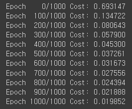
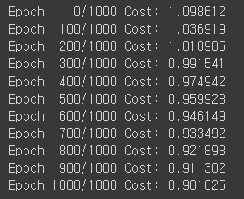
        print('Epoch {:4d}/{} Cost: {:.6f}'.format(
            epoch, nb_epochs, cost.item()
        ))

이전에 하였던 Linear Regression에서 학습했던 모델과 달라진점은 Hypothesis 와 cost방식만 바꿔주었습니다. W는 입력데이터는 2차원이며, 출력은 0아니면 1로 나오는 1차원의 데이터 입니다.
그렇기 때문에 W는 2행1열의 영행렬로 초기화 해주었으며 학습을 위한 변수로 사용하기 위해 requires_grad를 True로 설정해줍니다.

역시나 W와 b의 최적값을 찾기 위한 알고리즘으로 SGD를 사용하였고 learning rate를 1로 사용하였습니다.

binary classification 을 하기 위해서 hypothesis를 sigmoid를 사용하였으며 cost도 위와같은 Logistic을 사용하여 바꿔주었습니다.

그 후 backward시킨다는 의미는 cost를 다 계산하여 그 안에서 optimizer안에 있는 알고리즘을 수행한다는 것이고, optimizer.step()을 함으로써 W를 갱신합니다.

데이터 평가

hypothesis = torch.sigmoid(x_train.matmul(W) + b)
print(hypothesis[:5])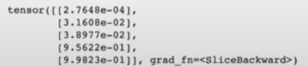

여기서 잘 학습된 W와 b를 구한 모델에 예측에 사용되었던 x_train 데이터를 다시 그 모델에 넣어 잘 학습이 되었는지 확인하기 위한 코드입니다.
예측을 한 뒤 5줄만 확인해봤을 때 0과 1이 아닌 이상한 값이 나오는 것을 알 수 있습니다.

Logistic Regression라고 하는 것은 범주형 데이터이기 때문에 이렇게 hypotheis에 예측한 값을 바로 출력하는 것이 아니라 이 값에서 0.5를 기준으로 크면 합격(1 or True), 작으면 불합격(0 or Flase)가 나오게 됩니다.

prediction = hypothesis >= torch.FloatTensor([0.5])

correct_prediction = prediction.float() == y_train
print(correct_prediction[:5])

accuracy = correct_prediction.sum().item() / len(correct_prediction)
print('The model has an accuracy of {:2.2f}% for the training set.'.format(accuracy * 100))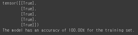

그렇게 0과 1로 재 레이블링을 하고난 후 원래 정답인 y_train과 비교해서 제대로 예측을 했는지 확인 해봅니다.
그랬을 때 상위 5줄 까지의 라벨링 예측은 모두 True라 정확도가 100%로 나오는 것을 확인할 수 있습니다.

이제는 학습된 데이터가 아니라 예측해보고자 하는 임의의 값을 넘어서 어떻게 예측하는지 확인해보겠습니다.

XX = [[100, 5]]
xx = torch.FloatTensor(XX);
hypothesis = torch.sigmoid(xx.matmul(W) + b)
prediction = hypothesis >= torch.FloatTensor([0.5])
print(prediction)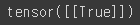

100시간 공부하고 5시간을 참석했다면 합격일까 불합격일까? 라는 예측을 해보았습니다.
그 결과 합격이라는 결과를 도출해내는 것을 확인했습니다.

---

이런 방식으로 스팸인지 아닌지, 고양인지 아닌지의 단 두가지 경우의 상황만 예측을하는 모델을 구현해보았습니다. 이제는 예측하고자 하는 결과값(라벨값)이 여러개인 예측을 해보겠습니다.

multi-classification

데이터 로더

import torch
import torch.optim as optim
# For reproducibility
torch.manual_seed(1)

x_train = [[1, 2, 1, 1],
           [2, 1, 3, 2],
           [3, 1, 3, 4],
           [4, 1, 5, 5],
           [1, 7, 5, 5],
           [1, 2, 5, 6],
           [1, 6, 6, 6],
           [1, 7, 7, 7]]
y_train = [2, 2, 2, 1, 1, 1, 0, 0]

x_train = torch.FloatTensor(x_train)
y_train = torch.LongTensor(y_train)

print(x_train[:5])   # 첫 다섯 개
print(y_train[:5])

y_train에 라벨값들을 보면 0과 1뿐만아니라 2라는 라벨값도 존재하여 3개 이상인 라벨값을 예측하는 분류 모델이라는걸 알 수 있습니다.
데이터 로더 부분은 Binary classification과 동일하게 텐서화를 시켜주었습니다.

모델 학습

import torch.nn.functional as F  # for softmax


# 모델 초기화
# feature 4개, 3개의 클래스
nb_class = 3
nb_data = len(y_train)

W = torch.zeros((4, nb_class), requires_grad=True)
b = torch.zeros(1, requires_grad=True)
# optimizer 설정
optimizer = optim.SGD([W, b], lr=0.01)
nb_epochs = 1000
for epoch in range(nb_epochs + 1):

    # Cost 계산 (1)
    hypothesis = F.softmax(x_train.matmul(W) + b, dim=1) # or .mm or @
    
    # cost 표현번 1번 예시
    y_one_hot = torch.zeros(nb_data, nb_class)
    y_one_hot.scatter_(1, y_train.unsqueeze(1), 1)
    cost = (y_one_hot * -torch.log(F.softmax(hypothesis, dim=1))).sum(dim=1).mean()
    
    # cost 표현법 2번 예시
    # cross_entropy를 사용하면 scatter 함수를 이용한 one_hot_encoding을 안해도 됨
    # cost = F.cross_entropy((x_train.matmul(W) + b), y_train)

    # cost로 H(x) 개선
    optimizer.zero_grad()
    cost.backward()
    optimizer.step()

    # 100번마다 로그 출력
    if epoch % 100 == 0:
        print('Epoch {:4d}/{} Cost: {:.6f}'.format(
            epoch, nb_epochs, cost.item()
        ))

feature(데이터 열의 개수)는 4개이며 class(라벨 개수)는 3개 이므로 W를 4행 3열의 영행렬을 만들어 주었습니다.
optimizer는 SGD로 동일하게 사용해주었고, 차이점은 가설설정에서 활성화함수를 Softmax를 사용하였다는 것입니다. (여기서 CrossEntropy를 그대로 사용하여도 좋고, 이렇게 Softmax를 직접 호출하여 사용해도 좋습니다.)

그 후 원한 잇코딩으로 y_train을 1열로 세우고 난후(y_train.unsqueeze(1)) cost를 위와같은 방식으로 계산을 해주었습니다.

데이터 평가

또 다시 우리가 만든 모델이 얼마나 잘 예측을 하는지 기존에 학습에 사용되었던 데이터인 x_train을 사용하여 확인을 해봅니다.

# 학습된 W,b를 통한 클래스 예측
hypothesis = F.softmax(x_train.matmul(W) + b, dim=1) # or .mm or @
predict = torch.argmax(hypothesis, dim=1)

torch.argmax()
print(hypothesis)
print(predict)
print(y_train)


# 정확도 계산 
correct_prediction = predict.float() == y_train
print(correct_prediction)
accuracy = correct_prediction.sum().item() / len(correct_prediction)
print('The model has an accuracy of {:2.2f}% for the training set.'.format(accuracy * 100))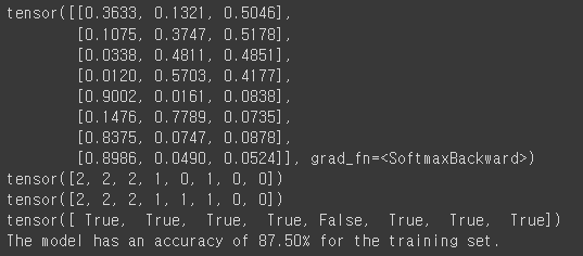

이렇게 나온 값은 첫번째 줄의 0.3633, 0.1321. 0.5046 에서 argmax함수를 통해 제일 큰 숫자의 인덱스의 값을 가져와 줍니다.

그 후 예측한 값과 실제 y_train값과 비교했을 때 86.5%의 정확도를 보이는 것을 확인했습니다.

---

여기까지 class가 여러개인 경우에도 Softmax라는 것을 이용해서 분류를 해내는 과정을 배웠습니다.
지금은 임의의 데이터로 하였지만 다음부터는 여러 공공데이터로 예측을 해보는 과정을 해볼 예정입니다.