Timeseries Anomaly Detection-(3) Unsupervised Learning

UnSupervised Learning

---

1. z-test

Check the distribution of datasets

# Check the distribution of the above stock data
fig, ax = plt.subplots(figsize=(9,6))
_ = plt.hist(df.Close, 100, density=True, alpha=0.75)

• Result
  

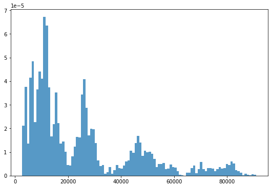
It does not follow a normal distribution.

from statsmodels.stats.weightstats import ztest

_, p = ztest(df.Close)
print(p)  # 0

If the value of p is less than 0.05, it means that it is far from the normal distribution, so it is difficult to analyze the confidence interval assuming the normal distribution with this data.

2) To extract data close to a normal distribution from a time series data set

from statsmodels.tsa.seasonal import seasonal_decompose

# Assume that the term of seasonality is 50 days
# extrapolate_trend='freq' : Because of the rolling window for creating a trend, the Nan value inevitably occurs in trend, resid. Therefore, it is an option that fills this NaN value.
result = seasonal_decompose(df.Close, model='additive', two_sided=True, 
                            period=50, extrapolate_trend='freq') 
result.plot()
plt.show()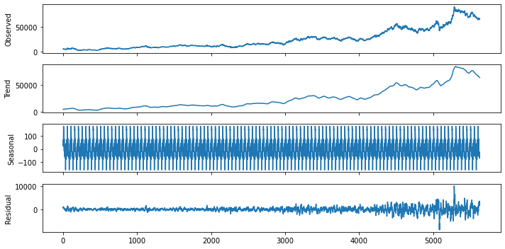

Check the 3rd Seasonal component in detail

result.seasonal[:100].plot()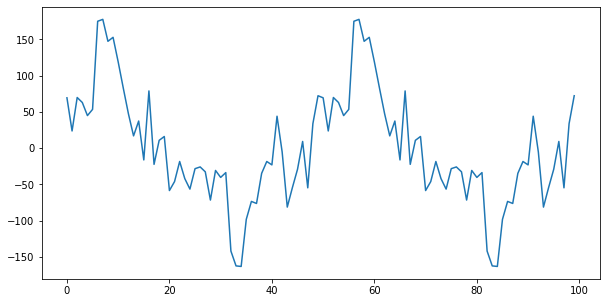

→ It can be seen that it repeats periodically between -160 and 180.

Since residuals are distributed based on an average of 0, days with large residuals can be interpreted as days out of general trend or seasonality.

# Check the distribution of Residual
fig, ax = plt.subplots(figsize=(9,6))
_ = plt.hist(result.resid, 100, density=True, alpha=0.75)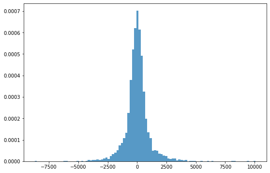

z-test (Check by number)

r = result.resid.values
st, p = ztest(r)
print(st,p)

Result
0.6948735022171139 0.4871345798943748

Since the value of p is more than 0.05 and the graph follows a normal distribution, the confidence interval analysis can be performed using this dataset.

# Output of Average and Standard Deviation 
mu, std = result.resid.mean(), result.resid.std()
print("평균:", mu)
print("표준편차:", std)


# Determine outliers based on 3-sigma (standard deviation)
print("이상치 갯수:", len(result.resid[(result.resid>mu+3*std)|(result.resid<mu-3*std)]))

#result:
#mean: 9.368886923797055
#standard deviation: 1011.6643445235127
#Number of outliers: 112

To view the details of 112 outliers

df.Date[result.resid[(result.resid>mu+3*std)|(result.resid<mu-3*std)].index]

4385   2017-05-08
4436   2017-07-20
4452   2017-08-11
4453   2017-08-14
4467   2017-09-04
          ...    
5619   2022-05-20
5620   2022-05-23
5625   2022-05-30
5626   2022-05-31
5628   2022-06-03
Name: Date, Length: 112, dtype: datetime64[ns]

Due to the explosion of Galaxy Note 7 in 2017 and the recent plunge in stock prices, abnormalities can be found.

# Data preprocessing
def my_decompose(df, features, freq=50):
    trend = pd.DataFrame()
    seasonal = pd.DataFrame()
    resid = pd.DataFrame()
    
    # Decompose for each feature to be used.
    for f in features:
        result = seasonal_decompose(df[f], model='additive', freq=freq, extrapolate_trend=freq)
        trend[f] = result.trend.values
        seasonal[f] = result.seasonal.values
        resid[f] = result.resid.values
        
    return trend, seasonal, resid

# Trends/seasonal/residuals for each variable
tdf, sdf, rdf = my_decompose(df, features=['Open','High','Low','Close','Volume'])
tdf.describe()

result

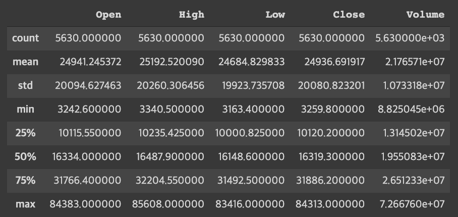
Trend by each variable

• Looking at the residuals for each variable, it can be seen that the value of the volume is particularly large compared to other values. If we use this data as it is, the volume will be reflected most importantly, so we can't get the exact value we want, so we give standard normalization.

# Standard normalization
from sklearn.preprocessing import StandardScaler

scaler = StandardScaler()
scaler.fit(rdf)
print(scaler.mean_)


norm_rdf = scaler.transform(rdf)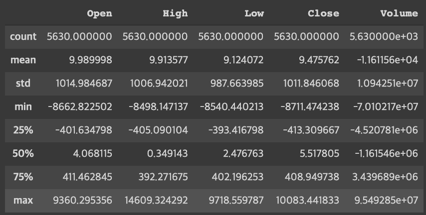
norm_rdf

result:
[ 9.98999848e+00  9.91357726e+00  9.12407232e+00  9.47576165e+00 -1.16115582e+04]
array([[ 0.91049378,  0.94485457,  0.76319233,  1.06571492,  2.06343412],
       [ 0.73231584,  0.91140349,  0.62369328,  0.56867739,  1.93682018],
       [ 0.66407391,  0.5997526 ,  0.64622584,  0.54419678, -0.03804234],
       ...,
       [ 2.80963702,  2.6765217 ,  2.93000737,  2.82886965, -0.09875707],
       [ 3.59222865,  3.16722954,  3.50891551,  3.09579198, -0.82225883],
       [ 2.75976516,  2.3669442 ,  2.24740122,  1.90013435,  0.28431761]])