[ML] 분류 모델 예측 평가 지표 공부하기

분류 성능 평가

1. 정확도 점수 (Accuracy Score)

• 정확도는 모델에서 올바르게 예측한 점수로 다음과 같다.
• 정확도 = (TP + TN) / (TP + TN + FP + FN)

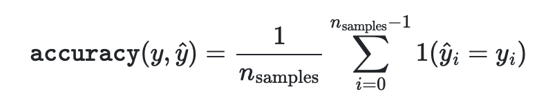
• yhat은 i 번째 예측 값이고, y는 실제 값이다.
• 따라서, yhat == y인 경우를 전체 경우로 나눈 경우이다.

기본 함수

from sklearn.metrics import accuracy_score
y_pred = [0, 2, 1, 3]
y_true = [0, 1, 2, 3]

accuracy_score(y_true, y_pred) <- 0.5임
accuracy_score(y_true, y_pred, normalize=False) <- 2임

• normalize = False를 하면 같은 경우의 셈을 의미한다.

Numpy 구현

import numpy as np

def accuracy_score(y_pred, y_true):
    yhat = np.array(y_pred)
    y = np.array(y_true)
    accuracy = np.mean(y == yhat)
    return accuracy

2. Top-k Accuracy Score

• 딥러닝 모델에서도 쓰이는 점수로 분류 모델에서 예측한 가장 가능성이 높은 N개의 클래스와 동일한 실제 클래스의 표준 정확도라고 할 수 있다.
• 예를 들어, 우리가 동물을 분류한다고 하자.

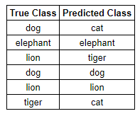
• 이 경우 우리는 50%의 정확도를 얻을 수 있다.

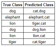
• 이 경우 각 예측값이 2개 이므로 83%의 정확도를 보여주고 있다.
• 이 처럼 정확도를 높이기 위해 예측 값의 개수를 늘리는 것을 Top-k 정확도라고 할 수 있다.

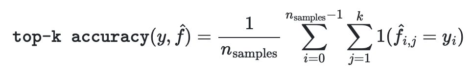
이 식을 보면서도 알 수 있는 것은 k개의 샘플을 일일이 대조하며 맞는 값을 찾으며 예측 정확도를 높이는 것이다.

기본 함수

import numpy as np
from sklearn.metrics import top_k_accuracy_score

y_true = np.array([0, 1, 2, 2])
y_score = np.array([[0.5, 0.2, 0.2],
                    [0.3, 0.4, 0.2],
                    [0.2, 0.4, 0.3],
                    [0.7, 0.2, 0.1]])

top_k_accuracy_score(y_true, y_score, k=2) <- 0.75임
top_k_accuracy_score(y_true, y_score, k=2, normalize=False) <- 3임

직접 구현

def top_k_accuracy(X, y, k, classifier):
    X_train, X_test, y_train, y_test = train_test_split(X, y, test_size=0.2)
    # 자연어처리 시 문자를 넣어 단어 출현 횟수를 세는 함수이다.
    vectorizer = TfidVectorizer(min_df=2)
    X_train_sparse = vectorizer.fit_transform(X_train)
    feature_names = vectorizer.get_feature_names()
    test = vectorizer.transform(X_test)
    clf = classifier
    clf.fit(X_train_sparse, y_train)
    predictions = clf.predict(test)
    probs = clf.predict_proba(test)
    # probs를 기준으로 정렬함
    topk = np.argsort(probs, axis = 1)[:, -n:]
    y_true = np.array(y_test)
    return np.mean(np.array([1 if y_true[k] in topk[k] else 0 for k in range(len(topk))]))

3. Balanced Accuracy Score

• 불균형 데이터 셋에서 과장된 성능 추정을 방지한다.
• 클래스당 재현율 점수의 매크로 평균이나 각 샘플이 실제 클래스의 역 보급에 따라 가중치가 부여되는 정확도라고 한다.
• 균형 잡힌 데이터 셋의 점수는 정확도와 같다.

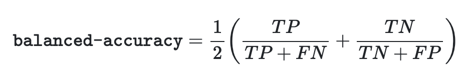
• Binary 경우에 Sensitivity(true positive rate)와 specificity (true negative rate)의 산술 평균으로 나타낼 수 있다.
• 예를 들어, 1000개의 라벨이 2개의 종류로 있을 때, Class1이 750개, Class2가 250개 그리고 예측률이 740/750 = 98.7%, 240//250=96%이면 아래처럼 나타남을 알 수 있다.

  Balanced_Accuracy_Score = (98.7%+96%)/2 = 97.35%

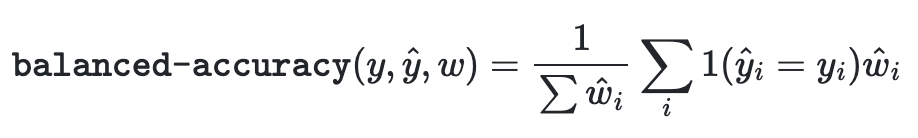
adjusted=True 의 경우 위에서 나타내는 1/nsamples이 1/(1- nsamples)로 불균형 데이터를 조정하려고 하는 것이 존재한다.

기본 함수

from sklearn.metrics import balanced_accuracy_score
y_true = [0, 1, 0, 0, 1, 0]
y_pred = [0, 1, 0, 0, 0, 1]
balanced_accuracy_score(y_true, y_pred)

Tensorflow 구현

class BalancedSparseCategoricalAccuracy(keras.metrics.SparseCategoricalAccuracy):
    def __init__(self, name='balanced_sparse_categorical_accuracy', dtype=None):
        super().__init__(name, dtype=dtype)

    def update_state(self, y_true, y_pred, sample_weight=None):
        y_flat = y_true
        if y_true.shape.ndims == y_pred.shape.ndims:
            y_flat = tf.squeeze(y_flat, axis=[-1])
        y_true_int = tf.cast(y_flat, tf.int32)

        cls_counts = tf.math.bincount(y_true_int)
        cls_counts = tf.math.reciprocal_no_nan(tf.cast(cls_counts, self.dtype))
        weight = tf.gather(cls_counts, y_true_int)
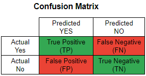
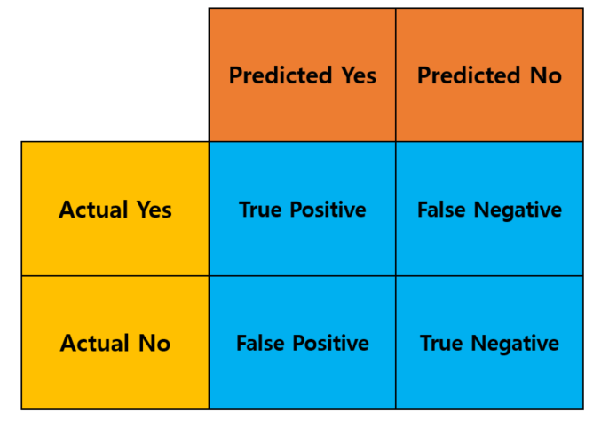
        return super().update_state(y_true, y_pred, sample_weight=weight)

4. Confusion Matrix

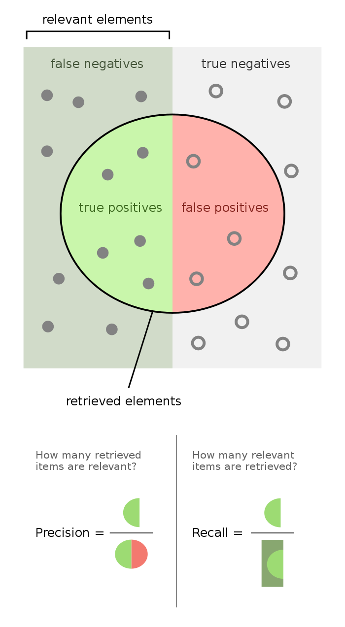
• 분류 모델을 평가하는 지표를 [TP, TN, FP, FN] 4가지로 구분하여 행렬로 나타낼 수 있는 지표를 말한다.

1. TP : 관심있는 지표를 정확하게 예측한 경우
2. TN : 관심없는 지표를 정확하게 예측한 경우
3. FP : 관심있는 지표를 잘못 예측한 경우
4. FN : 관심없는 지표를 잘못 예측한 경우

기본 함수

from sklearn.metrics import confusion_matrix

y_true = [2, 0, 2, 2, 0, 1]
y_pred = [0, 0, 2, 2, 0, 2]
confusion_matrix(y_true, y_pred)

출력
array([[2, 0, 0],
       [0, 0, 1],
       [1, 0, 2]])

Numpy 구현

import numpy as np

def compute_confusion_matrix(true, pred):
    # 고유값을 검색해 정렬함
    K = len(np.unique(true))
    
    # 고유값을 기준으로 KxK 행렬 생성
    result = np.zeros((K, K))
    
    for i in range(len(true)):
    	result[true[i]][pred[i]] += 1
    return result

5. Classification Report

classification_report는 분류 성능 평가에 필요한 지표를 text 형식의 Report로 지원해준다.

from sklearn.metrics import classification_report

y_true = [0, 1, 2, 2, 0]
y_pred = [0, 0, 2, 1, 0]
target_names = ['class 0', 'class 1', 'class 2']
print(classification_report(y_true, y_pred, target_names=target_names))

출력
              precision    recall  f1-score   support

     class 0       0.67      1.00      0.80         2
     class 1       0.00      0.00      0.00         1
     class 2       1.00      0.50      0.67         2

    accuracy                           0.60         5
   macro avg       0.56      0.50      0.49         5
weighted avg       0.67      0.60      0.59         5

6. Precision, recall

이진 분류 기업을 사용하는 곳에서 정밀도는 전체 예측 중에서 정확하게 예측한 비율이고, 재현율은 관련 있는 것들 중에서 실제 값들의 비율이다.

Precision, Recall 기본 함수

from sklearn.metrics import precision_score, recall_score
y_true = [0, 1, 2, 0, 1, 2]
y_pred = [0, 2, 1, 0, 0, 1]
precision_score(y_true, y_pred, average='macro')
recall_score(y_true, y_pred, average='weighted')

# average_precision_score 함수
import numpy as np
from sklearn.metrics import average_precision_score
y_true = np.array([0, 0, 1, 1])
y_scores = np.array([0.1, 0.4, 0.35, 0.8])
average_precision_score(y_true, y_scores)

Precision, Recall을 Python으로 구현하기

Case1

def compute_average_precision_recall(precision_recall_dict):
    precision = 0
    recall = 0
    for _, value in precision_recall_dict.items():
        precision += value['precision']
        recall += value['recall']
    average_precision = safe_divide(precision, len(precision_recall_dict))
    average_recall = safe_divide(recall, len(precision_recall_dict))
    return average_precision, average_recall

Case2 : Average_Precision

def compute_average_precision(precision, recall):
    precision = np.concatenate([[0.0], precision, [0.0]])
    for i in range(len(precision)-1, 0, -1):
        precision[i-1] = np.maximum(precision[i-1], precision[i])
    
    recall = np.concatenate([[0.0], recall, [1.0]])
    changing_points = np.where(recall[1:] != recall[:1][0])
    
    areas = (recall[changing_points + 1] - recall[changing_points]) * precision[changing_points + 1]
    return areas.sum()

7. F1-Score

F1-Score는 정밀도와 재현율의 조화평균으로 주로 분류 클래스 간 데이터가 심각한 불균형을 이루는 경우에 사용한다.

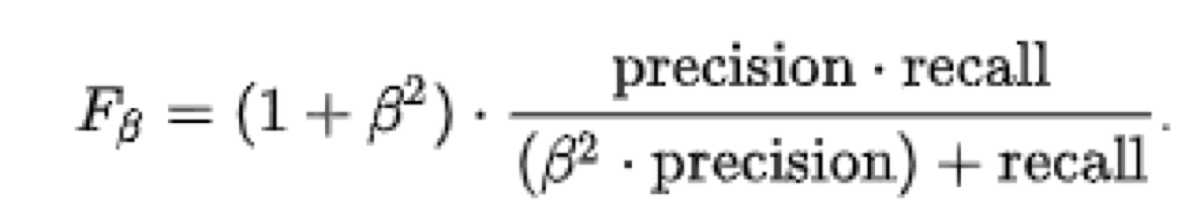
F1-Score는 여기서 베타 = 1인 경우로 보고 집어넣으면 된다.

기본 함수

from sklearn.metrics import f1_score
y_true = [0, 1, 2, 0, 1, 2]
y_pred = [0, 2, 1, 0, 0, 1]
f1_score(y_true, y_pred, average='macro')

f1-score with Macro로 구현하기

def f1(actual, predicted, label):
    tp = np.sum((actual==label) & (predicted==label))
    fp = np.sum((actual!=label) & (predicted==label))
    fn = np.sum((predicted!=label) & (actual==label))
    
    precision = tp/(tp+fp)
    recall = tp/(tp+fn)
    f1 = 2 * (precision * recall) / (precision + recall)
    return f1

def f1_macro(actual, predicted):
    return np.mean([f1(actual, predicted, label) 
        for label in np.unique(actual)])

8. ROC_CURVE 이해하기

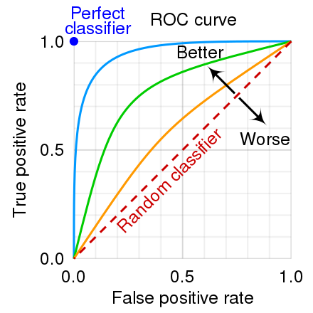
Roc_Curve를 보게 되면 X축은 FP, Y축은 TP로 얼마나 모델이 잘 분류를 하였는지 구분하며 Y축에 더 가까운 그래프를 형성할 수록 좋은 성능을 보인다고 말할 수 있다.

기본 함수

import numpy as np
from sklearn.metrics import roc_curve
y = np.array([1, 1, 2, 2])
scores = np.array([0.1, 0.4, 0.35, 0.8])
fpr, tpr, thresholds = roc_curve(y, scores, pos_label=2)

• FP, TP, 분류기준을 알 수 있다.