머신러닝 3주차

구글 Colab을 사용해 Python으로 머신러닝을 공부할 수 있다.

구글 드라이브 연동

구글 계정을 만들고 구글 드라이브에 들어가 Connect more apps를 클릭한다.

그리고 Colaboratory를 검색하고 설치한다. 위 그림은 이미 Colaboratory가 설치된 모습이다.

그럼 구글 드라이브에 Google Colaboratory 파일을 생성할 수 있다.

GitHub 연동

아래와 같이 구글 코랩에서 작업한 파일을 깃허브 저장소에 올릴 수 있다.

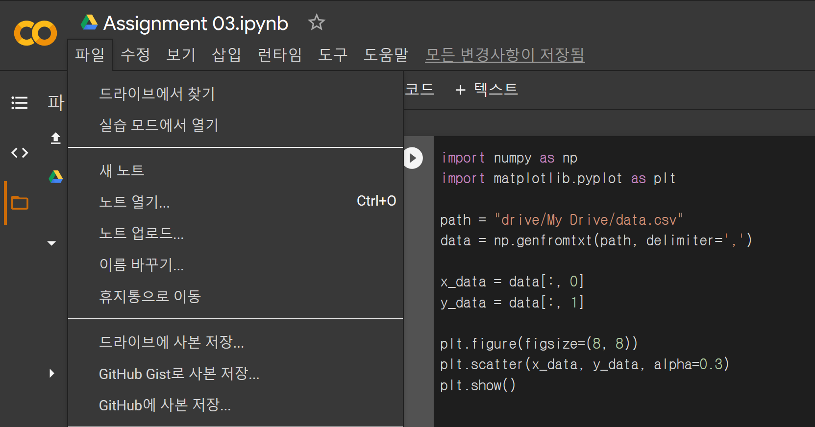
파일 ➞ GitHub에 사본 저장... ➞ GitHub 로그인

파일 ➞ GitHub에 사본 저장... ➞ 저장소, 브랜치, 파일 이름, 커밋 메시지 선택 ➞ 확인

구글 Colab에 파일 업로드

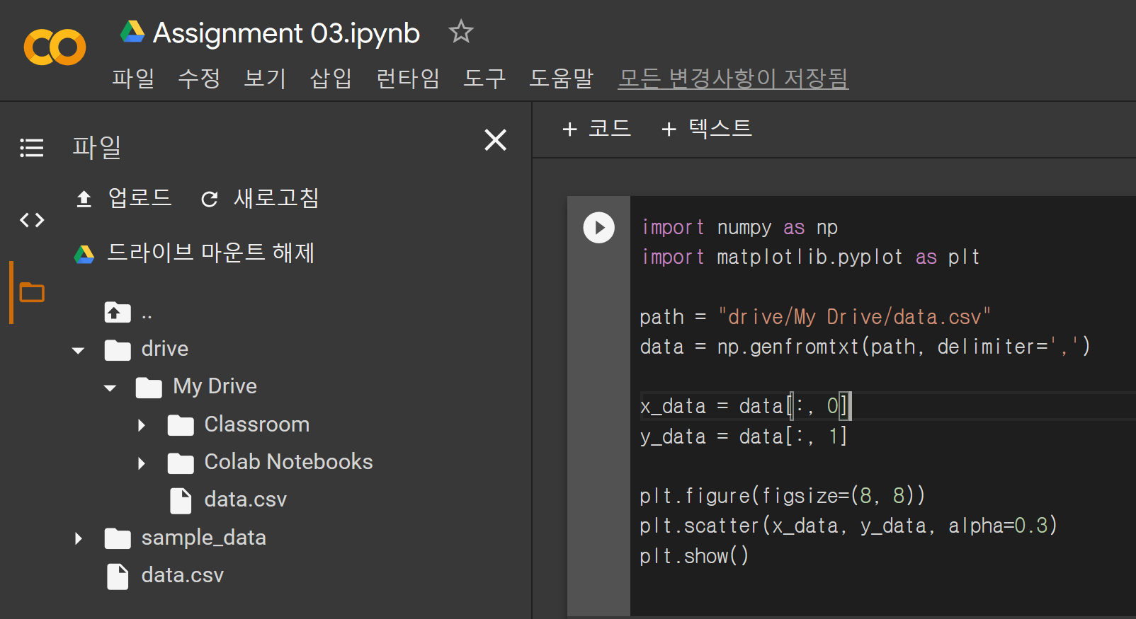
위 사진에서 업로드를 클릭하면 데이터 파일을 코랩에 업로드해서 불러올 수 있다. 하지만 업로드된 파일은 일정 시간이 지나서 연결이 끊기면 자동으로 사라지니 주의해야 한다.

또는 데이터 파일을 구글 드라이브에 올리고, 코랩에서 구글 드라이브를 마운트한 후 'drive/My Drive/.../data.csv'와 같은 경로로 데이터 파일을 불러올 수 있다.

머신러닝

1. 데이터 표현

import numpy as np
import matplotlib.pyplot as plt

# load data file
path = "drive/My Drive/.../data.csv"
data = np.genfromtxt(path, delimiter=',')

# get data set
x_data = data[:, 0]
y_data = data[:, 1]

# 1. Plot a set of points (xi, yi) that are loaded from 'data.csv' file (in black color)
plt.figure(figsize=(8, 8))
plt.scatter(x_data, y_data,color='black')
plt.show()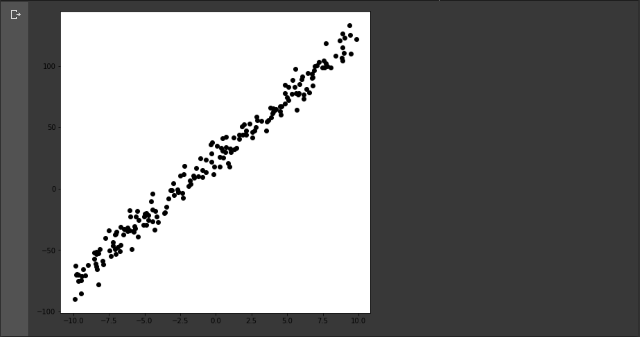

위와 같이 구글 드라이브에 올린 데이터 파일에서 데이터를 불러와서 화면에 표시할 수 있다. 데이터 셋의 형태는 아래와 같다.

• $(x_i, y_i)$ 의 리스트

2. 선형 회귀 분석

import numpy as np
import matplotlib.pyplot as plt
from math import isclose

# load data file
path = "drive/My Drive/.../data.csv"
data = np.genfromtxt(path, delimiter=',')

# get data set
x_data = data[:, 0]
y_data = data[:, 1]

# plot a set of points (xi, yi) that are loaded from 'data.csv' file (in black color)
plt.figure(figsize=(8, 8))
plt.scatter(x_data, y_data,color='black')

# Linear Function
def h(theta0, theta1, x):
  return theta0 + theta1 * x

# Objective Function
def J(theta0, theta1):
  sigma = 0
  for xi, yi in zip(x_data, y_data):
    sigma += (theta0 + theta1 * xi - yi) ** 2
  return (1 / (2 * len(x_data))) * sigma

# Derivative of Objective Function by theta0
def dJ_dtheta0(theta0, theta1):
  sigma = 0
  for xi, yi in zip(x_data, y_data):
    sigma += (h(theta0, theta1, xi) - yi)
  return (1 / len(x_data)) * sigma

# Derivative of Objective Function by theta1
def dJ_dtheta1(theta0, theta1):
  sigma = 0
  for xi, yi in zip(x_data, y_data):
    sigma += (h(theta0, theta1, xi) - yi) * xi
  return (1 / len(x_data)) * sigma

# Initial value of linear regression
theta0 = 100
theta1 = 100
learning_rate = 0.01

# get limit value of theta0 and theta1
while(1):
  next_theta0 = theta0 - learning_rate * dJ_dtheta0(theta0, theta1)
  next_theta1 = theta1 - learning_rate * dJ_dtheta1(theta0, theta1)

  # the gradient descent is performed until the convergence is achieved
  if(isclose(next_theta0, theta0) and isclose(next_theta1, theta1)):
    break

  # update theta0 and theta1
  theta0 = next_theta0
  theta1 = next_theta1

# 2. Plot a straight line obtained by the optimal linear regression based on the given set of points (in red color)
plt.plot([-10, 10], [h(theta0, theta1, -10), h(theta0, theta1, 10)], color='red')

# the estimated straight line (linear function) is superimposed on the set of points
plt.show()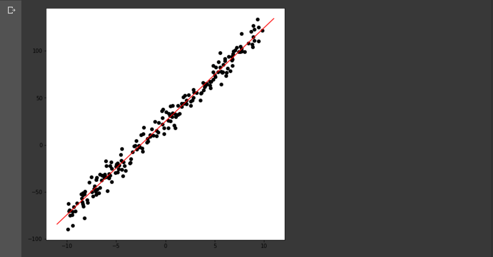

위와 같이 경사하강법을 통해 선형 회귀 분석을 할 수 있다. 과정은 아래와 같다.

1. 데이터 셋을 불러오고 선형 함수(1차 함수)를 설정한다.
   $h_\theta(x) = \theta_0 + \theta_1 x$

2. 목적 함수(에러 함수)를 설정한다. 우리는 이 목적 함수가 최소가 되게 하는 $\theta_0$, $\theta_1$을 구하려고 한다.
   $J(\theta_0, \theta_1) = \frac 1 {2m}\ \Sigma_{i=1}^m(\theta_0 + \theta_1 x_i - y_i)^2$

3. 경사하강법(Gradient Descent)으로 목적 함수가 최소가 되는 지점의 $\theta_0$, $\theta_1$을 찾아간다.
   ${\theta_0}_{i+1} = {\theta_0}_i - \alpha \frac {dJ({\theta_0}_i, {\theta_1}_i)} {d{\theta_0}_i}$, ${\lim\limits_{i\to\infin}{\theta_0}_i}$
   ${\theta_1}_{i+1} = {\theta_1}_i - \alpha \frac {dJ({\theta_0}_i, {\theta_1}_i)} {d{\theta_1}_i}$, ${\lim\limits_{i\to\infin}{\theta_1}_i}$

4. 경사하강법으로 구한 $\theta_0$, $\theta_1$을 선형 함수에 대입해 그래프로 그린다.

3. Energy surface 표현

import numpy as np
import matplotlib.pyplot as plt
from matplotlib import cm

# Objective Function
def J(theta0, theta1):
  sigma = 0
  for xi, yi in zip(x_data, y_data):
    sigma += (theta0 + theta1 * xi - yi) ** 2
  return (1 / (2 * len(x_data))) * sigma

# load data file
path = "data.csv"
data = np.genfromtxt(path, delimiter=',')

# get 2d points
x_data = data[:, 0]
y_data = data[:, 1]

# 3. Plot the energy surface
fig = plt.figure()
ax = fig.gca(projection='3d')

# plot the energy surface (theta0, theta1, J(theta0, theta1))
# with the range of variables theta0 = [−30:0.1:30] and theta1 = [−30:0.1:30]
theta0 = np.arange(-30, 30, 0.1)
theta1 = np.arange(-30, 30, 0.1)
theta0, theta1 = np.meshgrid(theta0, theta1)
surf = ax.plot_surface(theta0, theta1, J(theta0, theta1), rstride=10, cstride=10, cmap=cm.coolwarm, linewidth=0)

plt.show()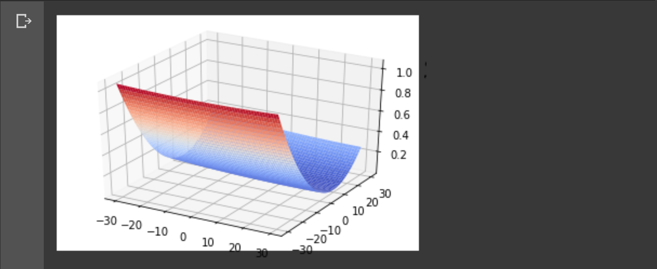

2차원 점을 불러와서 $(\theta_0, \theta_1,J(\theta_0, \theta_1))$을 3차원에 표현하면 저런 그래프가 나온다.

4. 선형 회귀 분석 경로 표현

import numpy as np
import matplotlib.pyplot as plt
from matplotlib import cm
from math import isclose

# load data file
path = "drive/My Drive/.../data.csv"
data = np.genfromtxt(path, delimiter=',')

# get 2d points
x_data = data[:, 0]
y_data = data[:, 1]

# Linear Model
def h(theta0, theta1, x):
  return theta0 + theta1 * x

# Objective Function
def J(theta0, theta1):
  sigma = 0
  for xi, yi in zip(x_data, y_data):
    sigma += (theta0 + theta1 * xi - yi) ** 2
  return (1 / (2 * len(x_data))) * sigma

# Derivative of Objective Function by theta0
def dJ_dtheta0(theta0, theta1):
  sigma = 0
  for xi, yi in zip(x_data, y_data):
    sigma += (h(theta0, theta1, xi) - yi)
  return (1 / len(x_data)) * sigma

# Derivative of Objective Function by theta1
def dJ_dtheta1(theta0, theta1):
  sigma = 0
  for xi, yi in zip(x_data, y_data):
    sigma += (h(theta0, theta1, xi) - yi) * xi
  return (1 / len(x_data)) * sigma

# 4. Plot the gradient descent path on the energy surface
fig = plt.figure()
ax = fig.gca(projection='3d')

# plot the energy surface (theta0, theta1, J(theta0, theta1))
# with the range of variables theta0 = [−30:0.1:30] and theta1 = [−30:0.1:30]
theta0 = np.arange(-30, 30, 0.1)
theta1 = np.arange(-30, 30, 0.1)
theta0, theta1 = np.meshgrid(theta0, theta1)
surf = ax.plot_surface(theta0, theta1, J(theta0, theta1), rstride=10, cstride=10, cmap=cm.coolwarm, linewidth=0)

# the initial condition is used by theta0 = -30 and theta1 = -30
theta0 = -30
theta1 = -30
learning_rate = 0.01
x = []
y = []
z = []

while(1):
  # plot the energy value with the updated variables theta0_i and theta1_i at each gradient descent step on the energy surface
  x.append(theta0)
  y.append(theta1)
  z.append(J(theta0, theta1))

  # get next thetas by the gradient descent method
  next_theta0 = theta0 - learning_rate * dJ_dtheta0(theta0, theta1)
  next_theta1 = theta1 - learning_rate * dJ_dtheta1(theta0, theta1)

  # the gradient descent is performed until the convergence is achieved
  if(isclose(next_theta0, theta0) and isclose(next_theta1, theta1)):
    break

  # update theta0 and theta1
  theta0 = next_theta0
  theta1 = next_theta1

# the gradient descent path is superimposed on the energy surface
ax.plot(x, y, z, marker="x", markeredgecolor="red")
ax.view_init(30, 30)
plt.show()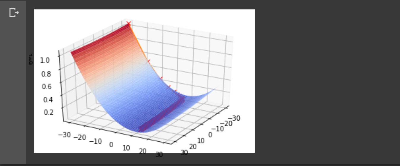

앞서 나온 코드랑 겹치는 부분이 많다. 차이점은 경사하강법으로 $\theta_0$과 $\theta_1$의 극한을 구할 때 그 값의 변화를 모두 저장해 energy surface 위에 표현한다는 점이다.