✅ 정확도 (Accuracy)
-
accuracy_score(y_test, y_pred) -
실제 데이터에서 예측 데이터가 얼마나 같은지를 판단하는 지표
-
분류의 경우, 데이터 구성에 따라 ML 모델의 성능을 왜곡할 수 있음
- 불균형한 레이블 값 분포에서 ML 모델의 성능을 판단할 경우, 적합한 평가지표가 아님
from sklearn.metrics import accuracy_score

print('정확도: {0:.4f}'.format(accuracy_score(y_test, y_pred))) # y_test: 실제값, y_pred: 예측값
✅ 오차행렬 (Confusion Matrix)
-
confusion_matrix(y_test, y_pred) -
학습된 분류 모델이 예측을 수행하면서 얼마나 헷갈리고 있는지 함께 보여주는 지표
-
앞 문자 True/False: 예측값과 실제값이 같은가/틀린가를 의미
-
뒤 문자 Negative/Positive: 예측 결과 값이 부정(0)/긍정(1)을 의미
-
매우 적은 수의 결괏값을 Positive(1)로 설정
- ex) 사기 행위 예측 모델: 사기 행위 양성(1), 정상 행위 음성(0)으로 정함
from sklearn.metrics import confusion_matrix

confusion_matrix(y_test, y_pred) # [[TN FP],
                                 #  [FN, TP]]
✅ 정밀도와 재현율
-
불균형한 데이터 세트에서 정확도보다 더 선호되는 평가 지표
-
Positive 데이터 세트의 예측 성능에 좀 더 초점을 맞춘 평가 지표
(1) 정밀도 (Precision)
-
precision_score(y_test, y_pred) -
TP / (FP+TP)
-
Positive를 예측한 것 중 맞춘 정도 = 양성 예측도
-
(음성을 양성으로 잘못 판단=FP) 낮추기
- ex) 스팸 메일 여부 판단 모델
(2) 재현율 (Recall)
-
recall_score(y_test, y_pred) -
TP / (FN+TP)
-
실제 Positive를 맞춘 정도 = 민감도, TPR
-
(양성을 음성으로 잘못 판단=FN) 낮추기
- ex) 암 판단 모델, 금융 사기 적발 모델
from sklearn.metrics import precision_score, recall_score

print("정밀도:", precision_score(y_test, y_pred))
print("재현율:", recall_score(y_test, y_pred))
(3) 정밀도/재현율 트레이드 오프 (Trade-off)
-
정밀도와 재현율은 상호 보완적인 평가 지표
-
어느 한쪽을 강제로 높이면 다른 하나의 수치는 떨어지기 쉬움
-
임곗값이 낮을수록 많은 수의 양성 예측으로 인해 재현율 값은 높아지고, 정밀도 값은 낮아진다.
-
임곗값이 높을수록 많은 수의 음성 예측으로 인해 정밀도 값은 높아지고, 재현율 값은 낮아진다.
-
-
binarizer=Binarizer(threshold): 임곗값(threshold) 지정 가능-
binarizer.fit() -
binarizer.predict()
-
from sklearn.preprocessing import Binarizer

# Binarizer의 threshold 설정값: 분류 결정 임곗값
custom_threshold = 0.5

# Positive 예측 확률 배열 적용
pred_proba_1 = pred_proba[:,1].reshape(-1,1)

binarizer = Binarizer(threshold=custom_threshold).fit(pred_proba_1)
custom_predict = binarizer.transform(pred_proba_1)
-
precision_recall_curve(y_test, Positive 예측 확률 배열)-
임곗값별 정밀도와 재현율을 구함
-
정밀도, 재현율, 임계값 반환
-
from sklearn.metrics import precision_recall_curve

# 레이블 값이 1일 때의 예측 확률을 추출
pred_proba_class1 = model.predict_proba(X_test)[:, 1]

precisions, recalls, thresholds = precision_recall_curve(y_test, pred_proba_class1 )

# 반환된 임계값 배열 중 샘플로 10건만 추출하되, 임곗값을 15 Step으로 추출
thr_index = np.arange(0, thresholds.shape[0], 15)
print('샘플 추출을 위한 임계값 배열의 index 10개:', thr_index)
print('샘플용 10개의 임곗값: ', np.round(thresholds[thr_index], 2))

# 15 step 단위로 추출된 임계값에 따른 정밀도와 재현율 값
print('샘플 임계값별 정밀도: ', np.round(precisions[thr_index], 3))
print('샘플 임계값별 재현율: ', np.round(recalls[thr_index], 3))
✅ F1 스코어
-
f1_score(y_test, y_pred) -
정밀도와 재현율을 결합한 지표
-
정밀도와 재현율이 어느 한 쪽으로 치우치지 않는 수치를 나타낼 때, 상대적으로 높은 값을 가짐
-
계산식: 2 X (정밀도 X 재현율) / (정밀도+재현율)
from sklearn.metrics import f1_score

print('F1 스코어: {0:.4f}'.format(f1_score(y_test, y_pred))) # y_test: 실제값, y_pred: 예측값
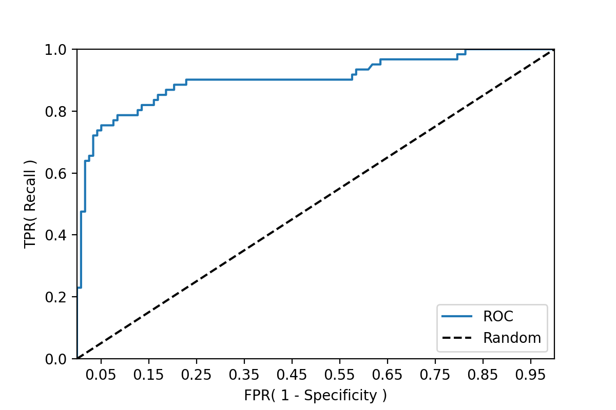
✅ ROC 곡선과 AUC
-
이진 분류의 예측 성능 측정에서 중요하게 사용되는 지표
-
ROC 곡선: FPR(X축)이 변할 때, TPR(Y축, 재현율=민감도)이 어떻게 변하는지를 나타내는 곡선
-
임계값을 1부터 0까지 거꾸로 변화시키면서 구한 재현율 곡선의 형태
-
TPR: 민감도, 실제값 Positive가 정확히 예측돼야 하는 수준
-
TNR: 특이성, 실제값 Negative가 정확히 예측돼야 하는 수준
-
FPR: (1-TNR) = (1-특이성)
-
-
AUC (Area Under Curve): ROC 곡선 밑의 면적
- 1에 가까울수록 좋은 수치
-
roc_curve(y_test, Positive 예측 확률 배열)- fpr, tpr, thresholds 반환
from sklearn.metrics import roc_curve

# 레이블 값이 1일때의 예측 확률을 추출
pred_proba_class1 = model.predict_proba(X_test)[:, 1]

fprs, tprs, thresholds = roc_curve(y_test, pred_proba_class1)

# 반환된 임곗값 배열 중 샘플 데이터를 추출하되, 임곗값을 5 Step으로 추출
# thresholds[0]은 max(예측확률)+1로 임의 설정, 이를 제외하기 위해 np.arange는 1부터 시작
thr_index = np.arange(1, thresholds.shape[0], 5)
print('샘플 추출을 위한 임곗값 배열의 index:', thr_index)
print('샘플 index로 추출한 임곗값: ', np.round(thresholds[thr_index], 2))

# 5 step 단위로 추출된 임계값에 따른 FPR, TPR 값
print('샘플 임곗값별 FPR: ', np.round(fprs[thr_index], 3))
print('샘플 임곗값별 TPR: ', np.round(tprs[thr_index], 3))
# ROC 곡선 시각화
def roc_curve_plot(y_test, pred_proba_c1):
    # 임곗값에 따른 FPR, TPR 값을 반환 받음.
    fprs , tprs , thresholds = roc_curve(y_test, pred_proba_c1)

    # ROC Curve를 plot 곡선으로 그림
    plt.plot(fprs, tprs, label='ROC')
    # 가운데 대각선 직선을 그림
    plt.plot([0, 1], [0, 1], 'k--', label='Random')

    # FPR X 축의 Scale을 0.1 단위로 변경
    start, end = plt.xlim()
    plt.xticks(np.round(np.arange(start, end, 0.1),2))
    plt.xlim(0,1); plt.ylim(0,1)

    # X,Y 축 제목
    plt.xlabel('FPR( 1 - Specificity )'); plt.ylabel('TPR( Recall )')
    plt.legend()
    plt.show()

roc_curve_plot(y_test, model.predict_proba(X_test)[:, 1])
roc_auc_score(y_test, Positive 예측 확률 배열)
from sklearn.metrics import roc_auc_score

# 레이블 값이 1일때의 예측 확률을 추출
pred_proba = model.predict_proba(X_test)[:, 1]

print('AUC: {0:.4f}'.format(roc_auc_score(y_test, pred_proba)))
