Pipeline

고은서·2023년 12월 17일

Data Preprocessing

목록 보기

9/10

10.1 파이프라인이란?

10.1.1 파이프라인

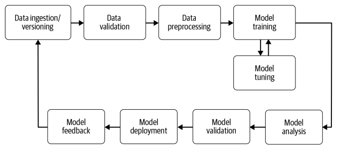
여러 개의 데이터의 처리(preprocessor, classifier, regressor, estimator 등)를 하나의 처리과정(pipeline, sequence)으로 만들어 데이터를 일괄처리해 주는 기능
- 데이터 전처리, 특성추출, 모델 학습 의 과정을 연속된 흐름으로 구성한다.
- 단계들은 서로 연결되어 있어, 한 단계의 출력이 다음 단계로 연결된다.
파이프라인을 사용하면 데이터 전처리나 모델 구축 과정 등을 더 짧은 코드로, 더 가시성 있게, 더 효율적으로 처리할 수 있음
- 가독성 및 유지 보수성 향상: 코드가 간결하게 작성되므로 전반적인 가독성이 향상
- 실험 및 반복 용이성: 여러 실험을 수행하거나 다양한 설정으로 모델을 시도하기에 용이함
- 자동화 및 일괄처리 가능
다양한 패키지에서 파이프라인을 지원하고 있음
데이터 프레임: Pandas, Polars
머신러닝: SciKit-Learn
딥러닝: TensorFlow, PyTorch

10.1.2 Scikt-Learn의 파이프라인

SciKit-Learn에서는 Pipeline 클래스를 통해 파이프라인을 구현할 수 있음
Pipeline 클래스는 여러 개의 추정기(estimator)를 하나의 추정기처럼 사용할 수 있도록 해 줌

파이프라인 사용 목적

편의성과 캡슐화
- 전체 데이터 처리 시퀀스에서 fit과 predict를 한 번만 적용하면 됨
통합된 하이퍼 파라미터 최적화
- grid search를 이용하여 한 번에 하이퍼 파라미터 최적화 가능
안전성 강화
- 교차검증(cross-validation)시 랜덤성에 의한 데이터의 통계적 특성이 변경되는 것을 방지하여 일관성을 유지할 수 있음
```
  
```

10.2 파이프라인 만들기

파이프라인 사용하지 않은 경우와 사용한 경우 비교해보기

10.2.1 파이프라인 사용하지 않은경우

from sklearn.feature_selection import SelectKBest, f_classif # 피처선택 메서드
from sklearn.preprocessing import StandardScaler # 데이터 표준화
from sklearn.tree import DecisionTreeClassifier # 의사결정나무 분류기
from sklearn.datasets import load_iris # iris 데이터세트

# iris 데이터세트 로드
X, y = load_iris(return_X_y=True)

## 피쳐 선택
feat_sel = SelectKBest(f_classif, k=2)
X_selected = feat_sel.fit_transform(X, y)
print('Selected features:', feat_sel.get_feature_names_out())

## 표준화
scaler = StandardScaler()
scaler.fit(X_selected)
X_transformed = scaler.transform(X_selected)
print('Standard Scaled: \n', X_transformed[:5, :])

## 모델 학습
clf = DecisionTreeClassifier(max_depth=3)
clf.fit(X_transformed, y)
print('Estimate : ', clf.predict(X_transformed)[:3])
print('Accuracy : ', clf.score(X_transformed, y))

Selected features: ['x2' 'x3']
Standard Scaled:
[[-1.34022653 -1.3154443 ][-1.34022653 -1.3154443 ]
[-1.39706395 -1.3154443 ][-1.2833891 -1.3154443 ]
[-1.34022653 -1.3154443 ]]
Estimate : [0 0 0]
Accuracy : 0.9733333333333334

10.2.2 파이프라인 사용하는 경우

파이프라인은 (key, value)의 리스트를 구성하여 만듦
파이프라인을 사용하면, 변환된 데이터를 별도로 저장하지 않고 연속적으로 사용하므로 속도가 개선되고 메모리가 절약됨

from sklearn.pipeline import Pipeline # 파이프라인 구성을 위한 함수
from sklearn.feature_selection import SelectKBest, f_classif # 피처선택 메서드
from sklearn.preprocessing import StandardScaler # 데이터 표준화
from sklearn.tree import DecisionTreeClassifier # 의사결정나무 분류기
from sklearn.datasets import load_iris # iris 데이터세트

# iris 데이터세트 로드
X, y = load_iris(return_X_y=True)

## pipeline 구축
pipeline = Pipeline([
    ('Feature_Selection', SelectKBest(f_classif, k=2)), ## 피쳐 선택
    ('Standardization', StandardScaler()),  ## 표준화
    ('Decision_Tree', DecisionTreeClassifier(max_depth=3)) ## 학습 모델
])
display(pipeline) # 파이프라인 그래프로 구성 확인

pipeline.fit(X, y) ## 모형 학습
print('Estimate : ', pipeline.predict(X)[:3]) ## 예측
print('Accuracy : ', pipeline.score(X, y)) ## 성능 평가

Estimate : [0 0 0]
Accuracy : 0.9733333333333334

make_pipeline()

make_pipeline() 함수를 사용하여 파이프라인을 만들 수 있음
- make_pipeline() 함수는 파이프라인의 이름을 자동으로 만들어 줌
- 파이프라인의 이름은 각 추정기의 클래스 이름을 소문자로 바꾼 것과 같음
- 파이프라인의 이름을 지정하려면 Pipeline() 클래스를 사용해야 함

from sklearn.pipeline import make_pipeline # 파이프라인 구성을 위한 함수

pipeline_auto = make_pipeline(SelectKBest(f_classif, k=2),
              StandardScaler(),
              DecisionTreeClassifier(max_depth=3))
display(pipeline_auto) # 파이프라인 그래프로 구성 확인

파이프라인 내부의 중간결과 확인하기

pipeline의 인덱스나 named_steps로 확인이 가능

# pipiline의 Feature_Selection step의 결과 확인
# pipeline.named_steps['Feature_Selection'] == pipeline[0]
# pipeline.named_steps['Standardization'] == pipeline[1]
# pipeline.named_steps['Decision_Tree'] == pipeline[2]
print('Selected features:', pipeline.named_steps['Feature_Selection'].get_feature_names_out())
X_transformed = pipeline[1].transform(X_selected)
print('Standard Scaled: \n', X_transformed[:5, :])

Selected features: ['x2' 'x3']
Standard Scaled:
[[-1.34022653 -1.3154443 ][-1.34022653 -1.3154443 ]
[-1.39706395 -1.3154443 ][-1.2833891 -1.3154443 ]
[-1.34022653 -1.3154443 ]]

10.3 파이프라인 결합

여러 파이프라인을 결합하여 전체 데이터 처리 프로세스를 정의할 수 있음

10.3.1 수치형데이터 파이프라인 처리

import seaborn as sns
import pandas as pd
from sklearn.pipeline import Pipeline
from sklearn.preprocessing import StandardScaler
from sklearn.impute import SimpleImputer

# 데이터 로드
df = sns.load_dataset('diamonds')
print(df.info())
X = df.drop('price', axis=1)
y = df['price']

# 데이터를 유형에 따라 분리
numeric_col = list(X.select_dtypes(exclude='category').columns)
category_col = list(X.select_dtypes(include='category').columns)
print(f'numeric_col: {numeric_col}')
print(f'category_col: {category_col}')

10.3.2 범주형 데이터 파이프라인처리

from sklearn.impute import SimpleImputer
from sklearn.preprocessing import OneHotEncoder

# 파이프라인 구축
category_pipeline = Pipeline(
    steps=[
        ('imputer', SimpleImputer(strategy='constant', fill_value='missing')), # 비어있는 값을 'missing'으로 채우기
        ('onehot', OneHotEncoder(sparse_output=False)), # Onehotencoder
    ])

display(category_pipeline) # 파이프라인 그래프로 구성 확인

# 파이프라인 학습
category_data_piped = category_pipeline.fit_transform(X[category_col])
# Onehotencoder의 컬럼명을 확인
category_colnames = category_pipeline[1].get_feature_names_out(category_col)
# 파이프라인 이후 데이터(array형 -> 데이터프레임)
pd.DataFrame(category_data_piped, columns=category_colnames).head()

10.3.3 수치형+범주형 결합한 파이프라인

from sklearn.compose import ColumnTransformer
from sklearn.linear_model import LinearRegression

# numeric & category 파이프라인 합치기
preprocessor = ColumnTransformer(
    transformers=[
        ('numeric', numeric_pipeline, numeric_col),
        ('category', category_pipeline, category_col)
    ])

pipe = make_pipeline(preprocessor, LinearRegression())
display(pipe) # 파이프라인 그래프로 구성 확인
pipe.fit(X,y)

print('Estimate : ', pipe.predict(X))
print('Accuracy : ', pipe.score(X, y))

10.3.4 Column Transformer

컬럼 기준으로 데이터를 복합하여 처리해주는 함수


from sklearn.compose import ColumnTransformer
from sklearn.impute import SimpleImputer
import pandas as pd
import numpy as np

data_df = pd.DataFrame({
    "height":[165,  np.nan, 182],
    "weight":[70,   62,     np.nan],
    "age"   :[np.nan,18,    15]
})

# SimpleImputer를 사용해서 height의 null 값들은 평균으로 출력하고 나머지 column은 통과
col_transformer = ColumnTransformer([
    ("Impute_mean", SimpleImputer(strategy="mean"), ["height"])
    ],
    remainder="passthrough"
)

display(col_transformer) # 파이프라인 그래프로 구성 확인
print(data_df)
print(col_transformer.fit_transform(data_df))

height weight age
0 165.0 70.0 NaN
1 NaN 62.0 18.0
2 182.0 NaN 15.0
[[165. 70. nan][173.5 62. 18. ]
[182. nan 15. ]]

# SimpleImputer를 사용해서 mean과 median 값을 null에 넣고
# 나머지 열(column)에 대한 값은 상수로 -1 값을 넣어 줌
col_transformer2 = ColumnTransformer([
    ("Impute_mean"  , SimpleImputer(strategy="mean")  , ["height"]),
    ("Impute_median", SimpleImputer(strategy="median"), ["weight"])
    ],
    remainder=SimpleImputer(strategy="constant", fill_value=-1)
)

display(col_transformer2) # 파이프라인 그래프로 구성 확인
print(data_df)
print(col_transformer2.fit_transform(data_df))