11. 불균형 데이터

11.1 불균형 데이터

불균형 데이터

• 분류 문제에서 타겟 데이터의 범주가 한 쪽으로 치우친 데이터
• 일반적으로 정상 데이터에 비해 이상 데이터가 매우 적은 경우
  - ex1. 양품 데이터에 비해 불량 데이터가 적은 경우
  • ex2. 중상 사고 데이터에 비해 사망사고 데이터가 적은 경우

불균형 데이터의 문제점

• 불균형 데이터는 모델의 성능을 왜곡시킨다
  - 정확도가 높아도, 이상 데이터는 검출해내지 못한다.
  • 정확도 외에 다른 성능 지표를 활용해야 한다.
• 이상 데이터에 과적합될 가능성이 높다.
  - 이상 데이터가 적기 때문에 이상 데이터에 과적합 될 가능성 높음
  

11.2 불균형 데이터의 해결방안

1. minority class 데이터를 추가 수집

• 현실적으로 수집이 어려움
• 수집에 시간과 비용이 많이 필요함
  

2. 모델의 성능 평가 지표를 변경

• 정확도 대신에 다른 성능 평가지표를 활용해야함
• Precision, Recall, F1-score, ROC-AUC, PR-AUC 등

3. 샘플링 기법으로 클래스별 데이터 균형을 맞춤

3.1 Undersampling

• majority class의 인스턴스를 일부만 사용하여 minority class의 인스턴스와 양적 균형을 맞춤
• 데이터 소실이 매우 크고, 중요한 정상 데이터를 잃을 수 있음

3.2 Oversampling

• minority class의 인스턴스를 복제 또는 유사 인스턴스를 생성하여 인스턴스수를 증가시키는 방법
• 정보가 손실되지 않는다는 장점이 있으나 과적합(Over-fitting)을 초래할 수 있음
  예)
• 인스턴스 복제: random over-sampling
• 유사 인스턴스 생성: SMOTE(Synthetic Minority Over-sampling Technique), ADASYN(Adaptive Synthetic Sampling Approach), Borderline-SMOTE

3.3 Undersampling + Oversampling 혼합

• majority class의 인스턴스는 일부만 사용하고 minority class의 인스턴스는 복제 또는 유사 인스턴스를 생성하여 균형을 맞춤
• 예) SMOTE + Tomek Links

4. 불균형 데이터에 강건한 모델 적용

• 앙상블(Ensemble) 모델 적용
  - 앙상블 모델은 서로 다른 여러 가지 모형들의 예측/분류 결과를 종합하여 최종적인 의사결정에 활용하는 기법
  - 여러 개의 모델을 학습할 때, 기존의 데이터를 균등하게 여러 데이터 셋으로 분류하여 학습을 수행
  - 과적합 감소효과 및 성능향상 가능
  - 예) Decision Tree, Random Forest, XGBoost, LightGBM, CatBoost, …

11.3 불균형 데이터 처리 방안

imbalanced learn 패키지

imbalanced-learn은 클래스 간 불균형을 보여주는 데이터 세트에서 일반적으로 사용되는 여러 리샘플링 기술을 제공하는 Python 패키지

다양한 샘플링 기법 비교

분류 문제 생성함수 정의

import warnings

# hide warnings
warnings.filterwarnings("ignore")

from sklearn.datasets import make_classification

# 분류 문제 데이터 생성하는 함수 정의, 독립변수 2개, 범주 x개
def create_dataset(n_samples, weights):
    return make_classification(
    n_samples=n_samples, 
    n_features=2, n_informative=2, n_redundant=0,
    n_classes=len(weights), n_clusters_per_class=1, weights=weights, 
    random_state=0)

결과 그래프 출력 함수 정의

import numpy as np
import matplotlib.pyplot as plt
import seaborn as sns

# 그래프 스타일 설정
sns.set_context("paper", font_scale=1)

# 분류기에 따른 결정영역을 표시하는 함수 정의 
def plot_decision_results(X, y, clf, ax, title=None):

    # 그리드 간격 설정
    grid_step = 0.02
    x_min, x_max = X[:, 0].min() - 1, X[:, 0].max() + 1   # X의 범위
    y_min, y_max = X[:, 1].min() - 1, X[:, 1].max() + 1   # y의 범위

    # meshgrid 함수를 사용하여 그리드 포인트 생성
    xx, yy = np.meshgrid(
        np.arange(x_min, x_max, grid_step), np.arange(y_min, y_max, grid_step)
    )

    # 예측 모델에 그리드 포인트 데이터를 입력하여 결정 영역을 계산
    # meshgrid 함수의 결과인 2차원 배열을 1차원 배열로 펼쳐서(.ravel()) 수평으로 쌓음(np.c_[])
    Z = clf.predict(np.c_[xx.ravel(), yy.ravel()])

    # 예측 결과를 그리드 포인트의 데이터 형태로 재배열
    Z = Z.reshape(xx.shape)

    # 그리드 포인트의 등고선을 그림
    ax.contourf(xx, yy, Z, alpha=0.4)

    # 클래스의 산점도를 그림
    ax.scatter(X[:, 0], X[:, 1], alpha=0.8, c=y, edgecolor="k")

    if title is not None:
        ax.set_title(title + f'\n({len(y[y==0])}, {len(y[y==1])}, {len(y[y==2])})', fontsize=12)

---

11.3.1 Undersampling

소수 클래스의 수를 고려하여 데이터 전체 표분의 크기를 축소시켜 균형을 맞추는 방법

1) Random UnderSampling

무작위로 majority class의 인스턴스를 제거하여 균형을 맞춤
샘플링시마다 결과가 다름

2) SMOTE(Synthetic Minority Over-Sampling Technique)

• majority class에서 중요하지 않은 인스턴스를 제거하는 것
• K-Means 알고리즘 활용
• 군집화(Clustering)하여 군집의 중심점(Centroid)을 찾고, 중심점과 가장 가까운 인스턴스만 보존

3) Edited Nearest Neighbours

• majority class 인스턴스 중 가장 가까운 k개의 인스턴스가 모두 또는 다수가 majority class가 아니면 삭제
• minority class 주변의 majority class 인스턴스는 삭제됨
• 주요 목적은 minority class 인스턴스의 분류 정확도를 높이는 것

4) Condensed Nearest Neighbour

• 1-NN(1-Nearest Neighbour) 알고리즘을 사용하여 1-NN 모형으로 분류되지 않는 인스턴스만 보존
• majority class에 밀집된 데이터가 없을 때까지 인스턴스를 제거하여 대표적인 인스턴스만 남도록 하는 방법

5) Tomek Links

서로 다른 클래스에 속하는 한 쌍의 인스턴스 중에서 가장 가까운 인스턴스(경계선에 있는 인스턴스)를 찾고, 그 중에서 majority class에 속하는 인스턴스를 제거

6) Near Miss

majority class에 속하는 인스턴스 중에서 minority class에 가까운 인스턴스를 보존

import numpy as np
from sklearn.linear_model import LogisticRegression
from imblearn.under_sampling import RandomUnderSampler, TomekLinks, EditedNearestNeighbours 
from imblearn.under_sampling import CondensedNearestNeighbour, NearMiss, ClusterCentroids

# 시드 설정
np.random.seed(0)

# 데이터 생성
X, y = create_dataset(n_samples=200, weights=(0.05, 0.25, 0.7))

# 샘플러 설정
samplers = [RandomUnderSampler(), 
            TomekLinks(),
            EditedNearestNeighbours(), 
            CondensedNearestNeighbour(n_neighbors=3),
            NearMiss(version=1, n_neighbors=3),
            NearMiss(version=2, n_neighbors=3),
            NearMiss(version=3, n_neighbors=3),
            ClusterCentroids()
            ]

# 서브 그래프 설정
fig, axs = plt.subplots(nrows=3, ncols=3, figsize=(10, 10))

# 분류기 생성
clf = LogisticRegression()

clf.fit(X, y)
plot_decision_results(X, y, clf, axs[0,0], title="Without resampling")

for i, sampler in enumerate(samplers):
    X_resampled, y_resampled = sampler.fit_resample(X, y)
    clf.fit(X_resampled, y_resampled)
    plot_decision_results(X_resampled, y_resampled, clf, axs[(i+1)//3,(i+1)%3], f"Using {sampler.__class__.__name__}")
    fig.suptitle(f"Decision function of {clf.__class__.__name__}")

fig.tight_layout()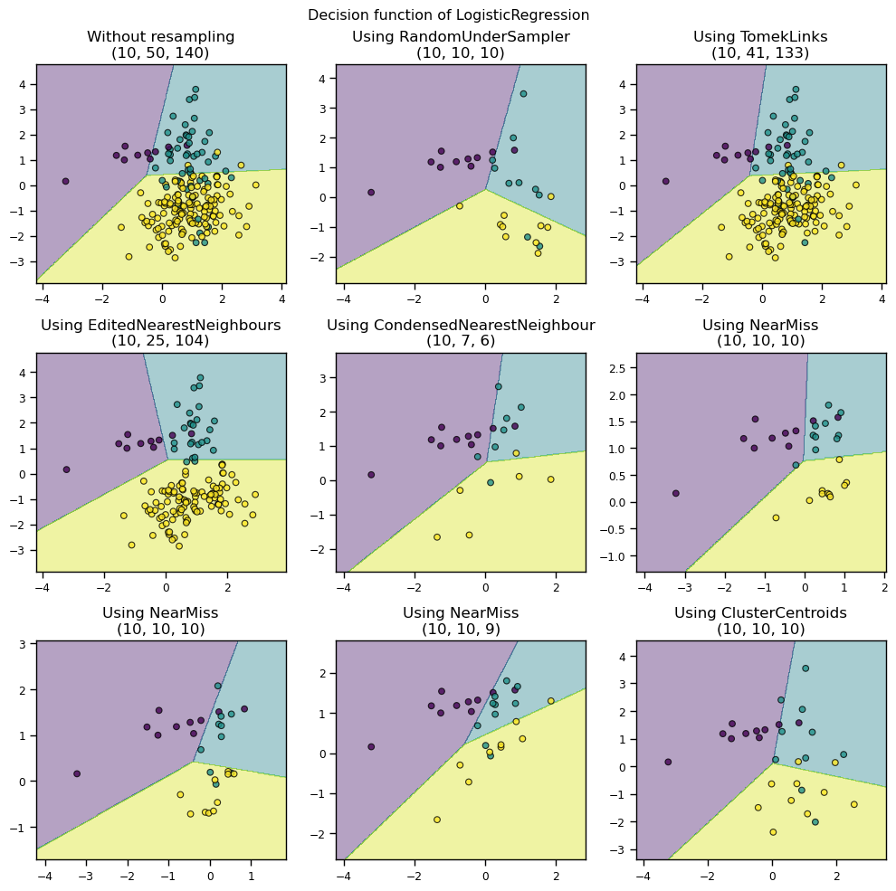

---

11.3.2 Oversampling

소수 클래스의 수를 다수 클래스의 수에 맞춰 증가시키는 방법

1) Random OverSampling

무작위로 minority class의 인스턴스를 복제하여 균형을 맞춤
동일하게 복제되기 때문에 과적합 발생에 주의해야함

2) SMOTE(Synthetic Minority Over-Sampling Technique)

각 minority class 인스턴스의 K-최근접 이웃을 찾고 그 중 하나를 무작위로 선택한 다음 선형 보간을 계산하여 이웃에 새로운 minority class 인스턴스를 생성
모델의 과적합을 방지하는데에 유용함

3) ADASYN (Adaptive Synthetic Sampling Approach)

모든 minority class 인스턴스에 대해 K-최근접 이웃을 측정한 다음 minority class 인스턴스와 majority class 인스턴스의 클래스 비율을 계산하여 새 인스턴스를 생성

4) Borderline-SMOTE

경계선(borderline)에 있는 인스턴스만 SMOTE를 적용

5) SVM-SMOTE

경계선(borderline)에 있는 인스턴스만 SMOTE를 적용

6) SMOTE + ENN

SMOTE를 사용하여 minority class의 데이터를 생성하고, 그 중에서 majority class에 속하는 데이터를 Edited Nearest Neighbours를 이용하여 제거

import numpy as np
from sklearn.linear_model import LogisticRegression
from imblearn.over_sampling import RandomOverSampler, SMOTE, ADASYN, BorderlineSMOTE, SVMSMOTE, KMeansSMOTE
from imblearn.combine import SMOTETomek, SMOTEENN

# 시드 설정
np.random.seed(0)

# 데이터 생성
X, y = create_dataset(n_samples=200, weights=(0.05, 0.25, 0.7))

# 샘플러 설정
samplers = [RandomOverSampler(),
            SMOTE(),
            ADASYN(),
            BorderlineSMOTE(),
            SVMSMOTE(),
            KMeansSMOTE(),
            SMOTETomek(),
            SMOTEENN()            
            ]

# 서브 그래프 설정
fig, axs = plt.subplots(nrows=3, ncols=3, figsize=(10, 10))

# 분류기 생성
clf = LogisticRegression()

clf.fit(X, y)
plot_decision_results(X, y, clf, axs[0,0], title="Without resampling")

for i, sampler in enumerate(samplers):
    X_resampled, y_resampled = sampler.fit_resample(X, y)
    clf.fit(X_resampled, y_resampled)
    plot_decision_results(X_resampled, y_resampled, clf, axs[(i+1)//3,(i+1)%3], f"Using {sampler.__class__.__name__}")
    fig.suptitle(f"Decision function of {clf.__class__.__name__}")

fig.tight_layout(pad=1.5)
plt.show()

---

11.3.3 Undersampling + Oversampling

1) SMOTE + Tomek Links

• SMOTE를 사용하여 minority class의 데이터를 생성하고, 그 중에서 majority class에 속하는 데이터를 Tomek Links를 이용하여 제거

2) SMOTE + ENN

• SMOTE를 사용하여 minority class의 데이터를 생성하고, 그 중에서 majority class에 속하는 데이터를 Edited Nearest Neighbours를 이용하여 제거

import numpy as np
from sklearn.linear_model import LogisticRegression
from imblearn.over_sampling import RandomOverSampler, SMOTE, ADASYN, BorderlineSMOTE, SVMSMOTE, KMeansSMOTE
from imblearn.combine import SMOTETomek, SMOTEENN

# 시드 설정
np.random.seed(0)

# 데이터 생성
X, y = create_dataset(n_samples=200, weights=(0.05, 0.25, 0.7))

# 샘플러 설정
samplers = [RandomOverSampler(),
            SMOTE(),
            ADASYN(),
            BorderlineSMOTE(),
            SVMSMOTE(),
            KMeansSMOTE(),
            SMOTETomek(),
            SMOTEENN()            
            ]

# 서브 그래프 설정
fig, axs = plt.subplots(nrows=3, ncols=3, figsize=(10, 10))

# 분류기 생성
clf = LogisticRegression()

clf.fit(X, y)
plot_decision_results(X, y, clf, axs[0,0], title="Without resampling")

for i, sampler in enumerate(samplers):
    X_resampled, y_resampled = sampler.fit_resample(X, y)
    clf.fit(X_resampled, y_resampled)
    plot_decision_results(X_resampled, y_resampled, clf, axs[(i+1)//3,(i+1)%3], f"Using {sampler.__class__.__name__}")
    fig.suptitle(f"Decision function of {clf.__class__.__name__}")

fig.tight_layout(pad=1.5)
plt.show()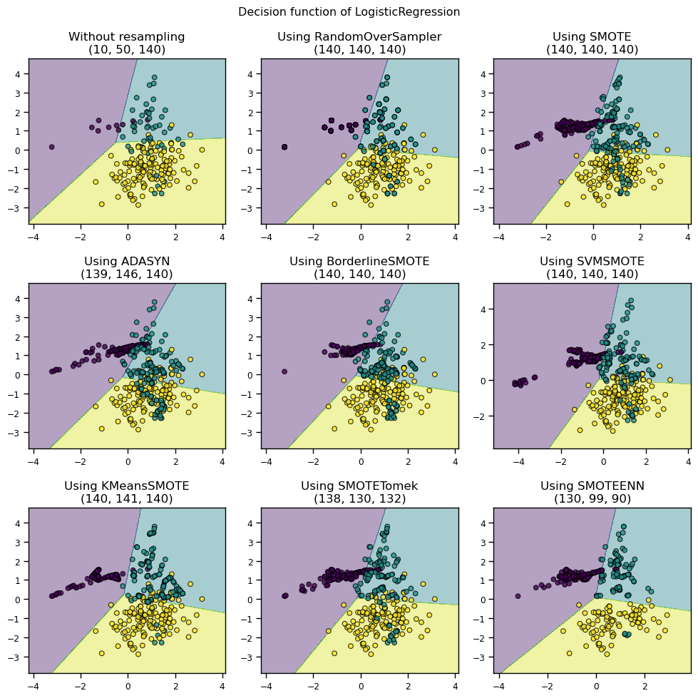

---

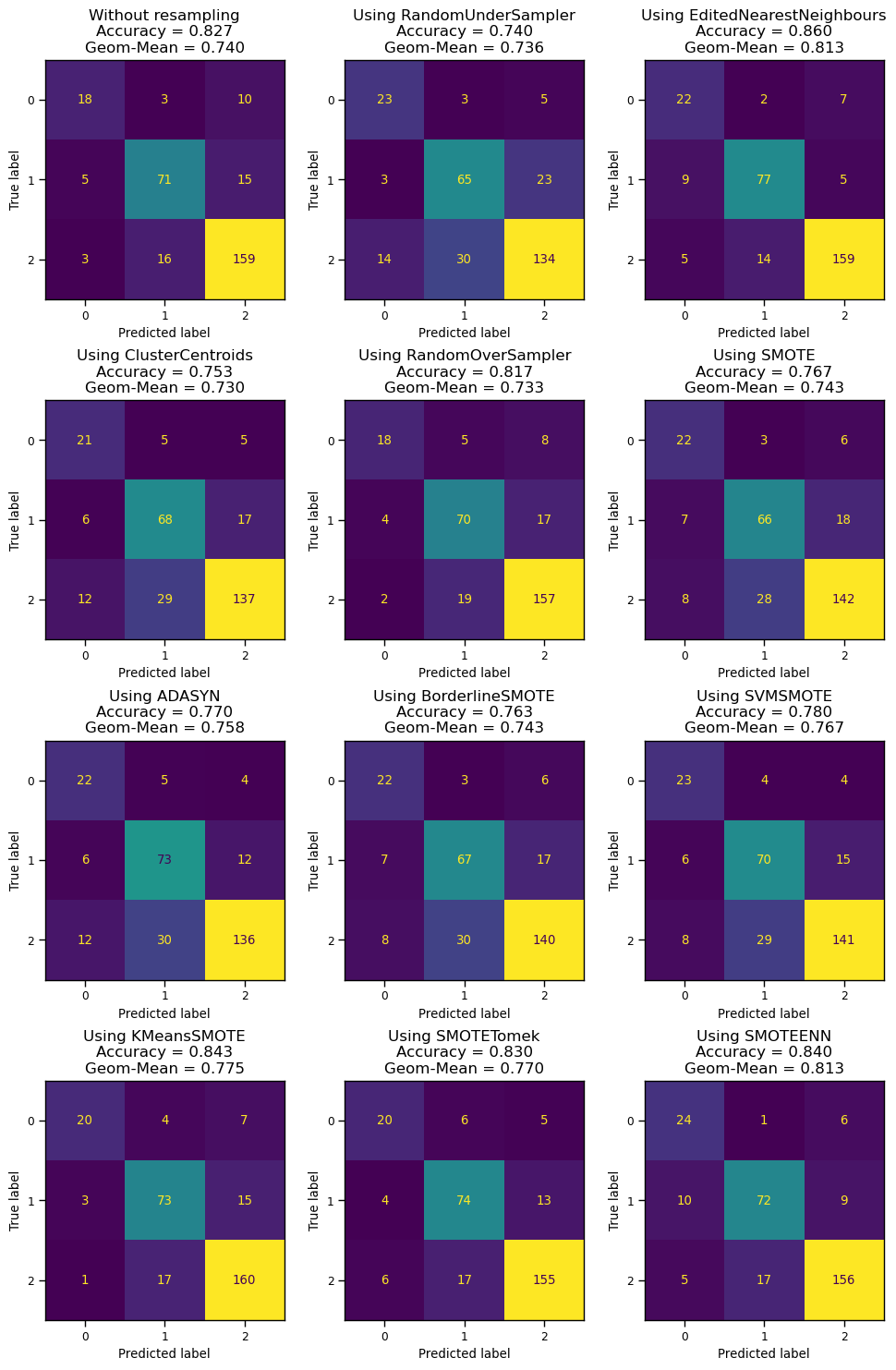
11.3.4 샘플링 기법 성능 비교

import numpy as np
from sklearn.metrics import ConfusionMatrixDisplay
from sklearn.model_selection import train_test_split
from sklearn.tree import DecisionTreeClassifier
from imblearn.under_sampling import RandomUnderSampler, TomekLinks, EditedNearestNeighbours, NearMiss, ClusterCentroids
from imblearn.over_sampling import RandomOverSampler, SMOTE, ADASYN, BorderlineSMOTE, SVMSMOTE, KMeansSMOTE
from imblearn.combine import SMOTETomek, SMOTEENN
from imblearn.metrics import geometric_mean_score

# 시드 설정
np.random.seed(0)

# 데이터 생성
X, y = create_dataset(n_samples=1000, weights=(0.1, 0.3, 0.6))
# 데이터셋 분리
X_train, X_test, y_train, y_test = train_test_split(X, y, stratify=y, test_size=0.3, random_state=0)

# 샘플러 설정
samplers = [RandomUnderSampler(),
            EditedNearestNeighbours(),
            ClusterCentroids(),
            RandomOverSampler(),
            SMOTE(),
            ADASYN(),
            BorderlineSMOTE(),
            SVMSMOTE(),
            KMeansSMOTE(),
            SMOTETomek(),
            SMOTEENN()
            ]

# 분류기 생성
clf = DecisionTreeClassifier()

# 서브 그래프 설정
fig, axs = plt.subplots(nrows=4, ncols=3, figsize=(10, 15))

clf.fit(X_train, y_train)
disp = ConfusionMatrixDisplay.from_estimator(clf, X_test, y_test, ax= axs[0,0], colorbar=False)
accuracy = clf.score(X_test, y_test)
geom_mean = geometric_mean_score(y_test, clf.predict(X_test))
disp.ax_.set_title(f"Without resampling\nAccuracy = {accuracy:.3f}\nGeom-Mean = {geom_mean:.3f}", fontsize=12)

for i, sampler in enumerate(samplers):
    X_resampled, y_resampled = sampler.fit_resample(X_train, y_train)
    clf.fit(X_resampled, y_resampled)
    accuracy = clf.score(X_test, y_test)
    geom_mean = geometric_mean_score(y_test, clf.predict(X_test))
    disp = ConfusionMatrixDisplay.from_estimator(clf, X_test, y_test, ax=axs[(i+1)//3,(i+1)%3], colorbar=False)
    disp.ax_.set_title(f"Using {sampler.__class__.__name__}\nAccuracy = {accuracy:.3f}\nGeom-Mean = {geom_mean:.3f}", fontsize=12)

fig.tight_layout(pad=2.0)
plt.show()

![](https://velog.velcdn.com/images/happycherry6/post/9438b5ce-878d-4d8b-98f3-4218791ca5f7/image.png)

---

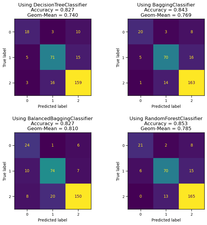
11.3.5 앙상블 방법 적용

import numpy as np
from sklearn.metrics import ConfusionMatrixDisplay
from sklearn.model_selection import train_test_split
from sklearn.tree import DecisionTreeClassifier
from sklearn.ensemble import BaggingClassifier, RandomForestClassifier
from imblearn.ensemble import BalancedBaggingClassifier, BalancedRandomForestClassifier
from imblearn.under_sampling import RandomUnderSampler, TomekLinks, EditedNearestNeighbours, NearMiss, ClusterCentroids
from imblearn.over_sampling import RandomOverSampler, SMOTE, ADASYN, BorderlineSMOTE, SVMSMOTE, KMeansSMOTE
from imblearn.combine import SMOTETomek, SMOTEENN
from imblearn.metrics import geometric_mean_score

# 시드 설정
np.random.seed(0)

# 데이터 생성
X, y = create_dataset(n_samples=1000, weights=(0.1, 0.3, 0.6))
# 데이터셋 분리
X_train, X_test, y_train, y_test = train_test_split(X, y, stratify=y, test_size=0.3, random_state=0)

# 분류기 생성
clfs = [DecisionTreeClassifier(),
        BaggingClassifier(n_estimators=50),
        BalancedBaggingClassifier(n_estimators=50),
        RandomForestClassifier(n_estimators=50)
        ]

# 서브 그래프 설정
fig, axs = plt.subplots(nrows=2, ncols=2, figsize=(8, 8))

for i, clf in enumerate(clfs):
    clf.fit(X_train, y_train)
    accuracy = clf.score(X_test, y_test)
    geom_mean = geometric_mean_score(y_test, clf.predict(X_test))
    disp = ConfusionMatrixDisplay.from_estimator(clf, X_test, y_test, ax=axs[i//2,i%2], colorbar=False)
    disp.ax_.set_title(f"Using {clf.__class__.__name__}\nAccuracy = {accuracy:.3f}\nGeom-Mean = {geom_mean:.3f}", fontsize=12)

fig.tight_layout(pad=2.0)
plt.show()