[정보 이론] KL-Divergence 측정

Reference

• https://machinelearningmastery.com/divergence-between-probability-distributions/
• https://angeloyeo.github.io/2020/10/26/information_entropy.html

1. Statistical Distance

There are many situations where we may want to compare two probability distributions.

Specifically, we may have a single random variable and two different probability distributions for the variable, such as a true distribution and an approximation of that distribution.

In situations like this, it can be useful to quantify the difference between the distributions.Generally, this is referred to as the problem of calculating the statistical distance between two statistical objects, e.g. probability distributions.

Note) the definition of 'distance' here is not same with the Euclidean distance, rather it focuses on the difference($\triangle$) between the different probability distributions)

One approach is to calculate a distance measure between the two distributions. This can be challenging as it can be difficult to interpret the measure.

Instead, it is more common to calculate a divergence between two probability distributions. A divergence is like a measure but is not symmetrical. $\rightarrow$ This means that a divergence is a scoring of how one distribution differs from another, where calculating the divergence for distributions P and Q would give a different score from Q and P.

$i,e.$ $\:$ $D_{KL}(P||Q)$ $\neq$ $D_{KL}(Q||P)$)

Divergence scores are an important foundation for many different calculations in information theory and more generally in machine learning. For example, they provide shortcuts for calculating scores such as mutual information (information gain) and cross-entropy used as a loss function for classification models.

Divergence scores are also used directly as tools for understanding complex modeling problems, such as approximating a target probability distribution when optimizing generative adversarial network (GAN) models.

Two commonly used divergence scores from information theory are Kullback-Leibler Divergence and Jensen-Shannon Divergence.

We will take a closer look at both of these scores in the following section.

2. Estimation of KL Divergence

2.1. Information Entropy Formula

Suppose there is a discrete random varible $X$ which has a sample sapce of ${x_1, x_2, ..., X_n}$, the entropy of information can be calculated with this formula which is simllar to a form of expected value($\sum_{i\in N}p_{i}x_{i}$.

$H(X) \: = E[(I(X))] \: = -\sum^{n}_{i=1}P(x_i)log_{b}(P(x_i))$ = $\sum^{n}_{i=1}P(x_i)log_{b}\frac{1}{P(x_i)}$

$where \: I(X) \: = \: Information \:of\:X$

2.2. KL Divergence Formula

$D_{KL}(P||Q)\:=\:\sum_{x \in X}p(x)log_{b}(\frac{P(x)}{Q(x)})$

Here, $2, \: 10 \:$, or $e$ are widely used as base numbers of $log$ function. Considering each base number case, the units of information are independently $bit$, $dit$, and $nit$.

Also, after the sigma, we can easily check a process which calculates the sum of difference between two expected values.

$\sum_{x \in X}(p(x)log_b(P(x))-p(x)log_b(Q(x))$

Regarding this, now we can understand the definition of "statistical distance" at the first part of this article.

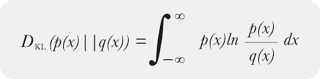
If a random variable is not a discrete(i.e, continuous random variable), we can use this Probability Density Function instead.

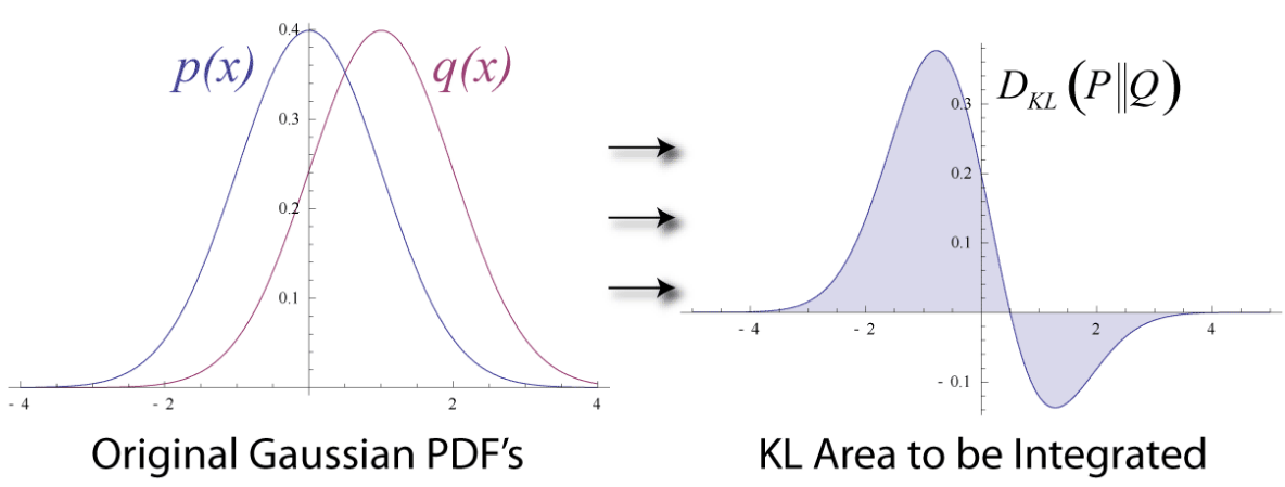
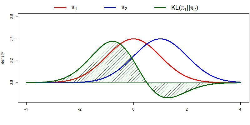
2.2.1. Visualization of KL Divergence

2.3. Implementation

define distributions $(P, Q)$

events = ['red', 'green', 'blue']
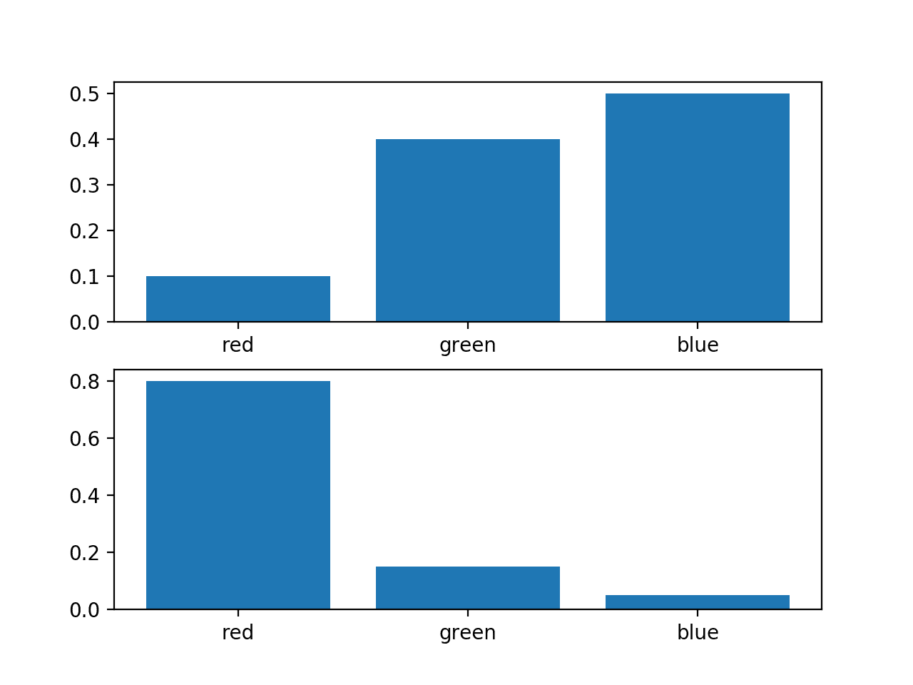
p = [0.10, 0.40, 0.50]
q = [0.80, 0.15, 0.05]

Let's define two random variables, p and q which are mapped with the three different events(domain of the probability distribution).

# plot of distributions
from matplotlib import pyplot
print('P=%.3f Q=%.3f' % (sum(p), sum(q)))

# plot first distribution
pyplot.subplot(2,1,1)
pyplot.bar(events, p)

# plot second distribution
pyplot.subplot(2,1,2)
pyplot.bar(events, q)

# show the plot
pyplot.show()

$P$ and $Q$ have those shapes of probability distribution below.

Let's estimate $D_{KL}(P || Q), \: D_{KL}(Q||P)$

# define the kl divergence with importing log2

from math import log2

def kl_divergence(p, q):
 return sum(p[i] * log2(p[i]/q[i]) for i in range(len(p)))

# define distributions
p = [0.10, 0.40, 0.50]
q = [0.80, 0.15, 0.05]

# calculate (P || Q)
kl_pq = kl_divergence(p, q)
print(f'KL(P || Q): {kl_pq} bits')

# calculate (Q || P)
kl_qp = kl_divergence(q, p)
print(f'KL(Q || P): {kl_qp} bits')

[Results : both results are different with each other !!]
KL(P || Q): 1.927 bits
KL(Q || P): 2.022 bits