[Tensorflow] 3. Natural Language Processing in TensorFlow (2 week Word Embeddings) : Programming (2)

[Tensorflow] 3. Natural Language Processing in TensorFlow (2 week Word Embeddings) : Programming (2)

Sarcasm 데이터 세트를 사용하여 이진 분류기 학습

• Programming (1) 에서는 imdb의 뉴스 헤드라인 기사를 통해서 긍정, 부정 분류기를 만들었다면 여기서는 지난주의 풍자 감지를 위한 뉴스 헤드라인 데이터 세트를 다시 방문하고 이에 대한 학습 모델을 구축하는 과정을 진행한다.
• 이 단계는 약간의 수정만 제외하면 이전 IMDB 리뷰 랩과 매우 유사하다. 여기서는 하이퍼파라미터를 조정해서 결과가 어떻게 변하는 지에 대해서 살펴본다.

[1] Download the dataset

import requests

url = 'https://storage.googleapis.com/tensorflow-1-public/course3/sarcasm.json'
filename = 'sarcasm.json'

response = requests.get(url)

with open(filename, 'wb') as f:
    f.write(response.content)

import json

with open('./'+filename, 'r') as f:
    datastore = json.load(f)
    
datastore[0]

# output
{'article_link': 'https://www.huffingtonpost.com/entry/versace-black-code_us_5861fbefe4b0de3a08f600d5',
 'headline': "former versace store clerk sues over secret 'black code' for minority shoppers",
 'is_sarcastic': 0}

로드한 데이터를 sentences 와 labels 데이터로 구분한다.

sentences =[]
labels = []

for item in datastore:
    sentences.append(item['headline'])
    labels.append(item['is_sarcastic'])
    
print(len(sentences))
print(len(labels))

# output
26709
26709

[2] Hyperparameters

training_size = 20000
vocab_size = 10000
max_length = 32
embedding_dim = 16

[3] split the dataset

다음으로 학습 및 테스트 데이터 세트를 생성한다.
위에서 설정한 training_size 값을 사용하여 문장과 레이블 목록을 두 개의 하위 목록(하나는 사전 훈련용, 다른 하나는 테스트용)으로 분할한다.

import numpy as np


training_sentences = sentences[0:training_size]
training_labels = labels[0:training_size]

testing_sentences = sentences[training_size:]
testing_labels = labels[training_size:]

[4] Preprocessing the train and test sets

이제 모델에서 사용할 수 있도록 텍스트와 레이블을 전처리할 수 있다. Tokenizer 클래스를 사용하여 어휘를 생성하고 pad_sequences 메서드를 사용하여 패딩된 토큰 시퀀스를 생성한다.
또한 model.fit()에 유효한 데이터 유형이 될 수 있도록 레이블을 numpy 배열로 설정한다.

from tensorflow.keras.preprocessing.text import Tokenizer
from tensorflow.keras.preprocessing.sequence import pad_sequences


tokenizer = Tokenizer(num_words=vocab_size, oov_token='<OOV>')

tokenizer.fit_on_texts(training_sentences)
word_index = tokenizer.word_index

train_sequences = tokenizer.texts_to_sequences(training_sentences)
train_padded = pad_sequences(train_sequences, truncating='post', maxlen=max_length)


test_sequences = tokenizer.texts_to_sequences(testing_sentences)
test_padded = pad_sequences(test_sequences, maxlen=max_length, truncating='post')

training_labels_final = np.array(training_labels)
testing_labels_final = np.array(testing_labels)

[5] Build and Compile the Model

다음으로 모델을 빌드한다.

아키텍처는 이전 실습과 유사하지만 포함 후 Flatten 대신 GlobalAveragePooling1D 레이어를 사용한다. 이는 조밀한 레이어에 연결하기 전에 시퀀스 차원에 대한 평균을 계산하는 작업을 추가한다.

최종 출력에 도달하기 위해 3개 배열(예: (10 + 1 + 1) / 3 및 (2 + 3 + 1) / 3)에 대한 평균을 얻는 것이다.

import tensorflow as tf

# Initialize a GlobalAveragePooling1D (GAP1D) layer
gap1d_layer = tf.keras.layers.GlobalAveragePooling1D()

# Define sample array
sample_array = np.array([[[10,2],[1,3],[1,1]]])

# Print shape and contents of sample array
print(f'shape of sample_array = {sample_array.shape}')
print(f'sample array: {sample_array}')

# Pass the sample array to the GAP1D layer
output = gap1d_layer(sample_array)

# Print shape and contents of the GAP1D output array
print(f'output shape of gap1d_layer: {output.shape}')
print(f'output array of gap1d_layer: {output.numpy()}')

# output

shape of sample_array = (1, 3, 2)
sample array: [[[10  2]
  [ 1  3]
  [ 1  1]]]
output shape of gap1d_layer : (1, 2)
output array of gap1d_layer : [[4. 2.]]

기존에는 Flatten()을 사용했지만 GlobalAveragePooling1D() 을 사용해서 모델을 빌드한다.

import tensorflow as tf


model = tf.keras.models.Sequential([
    tf.keras.layers.Embedding(vocab_size, embedding_dim, input_length=max_length),
    tf.keras.layers.GlobalAveragePooling1D(),
    tf.keras.layers.Dense(24, activation='relu'),
    tf.keras.layers.Dense(1, activation='sigmoid')
    
])

model.compile(loss='binary_crossentropy',
              optimizer='adam',
              metrics=['accuracy'])

이제 준비된 데이터세트를 입력하여 모델을 훈련한다.
기본 하이퍼파라미터를 사용한 경우 약 99%의 훈련 정확도와 80%의 검증 정확도를 얻을 수 있다.

• model.fit()의 verbose 매개변수를 2로 설정하여 에포크당 결과만 인쇄하려는 것을 나타낼 수 있습니다. 1(기본값)로 설정하면 에포크당 진행률 표시줄이 표시되고, 0으로 설정하면 모든 표시가 나오지 않는다. 프로덕션 환경에서 작업할 때는 문서에서 권장하는 대로 이 값을 2로 설정하는 것이 좋습니다.

https://keras.io/api/models/model_training_apis/#fit-method

history = model.fit(train_padded, training_labels_final, epochs=30,
          validation_data = (test_padded, testing_labels_final))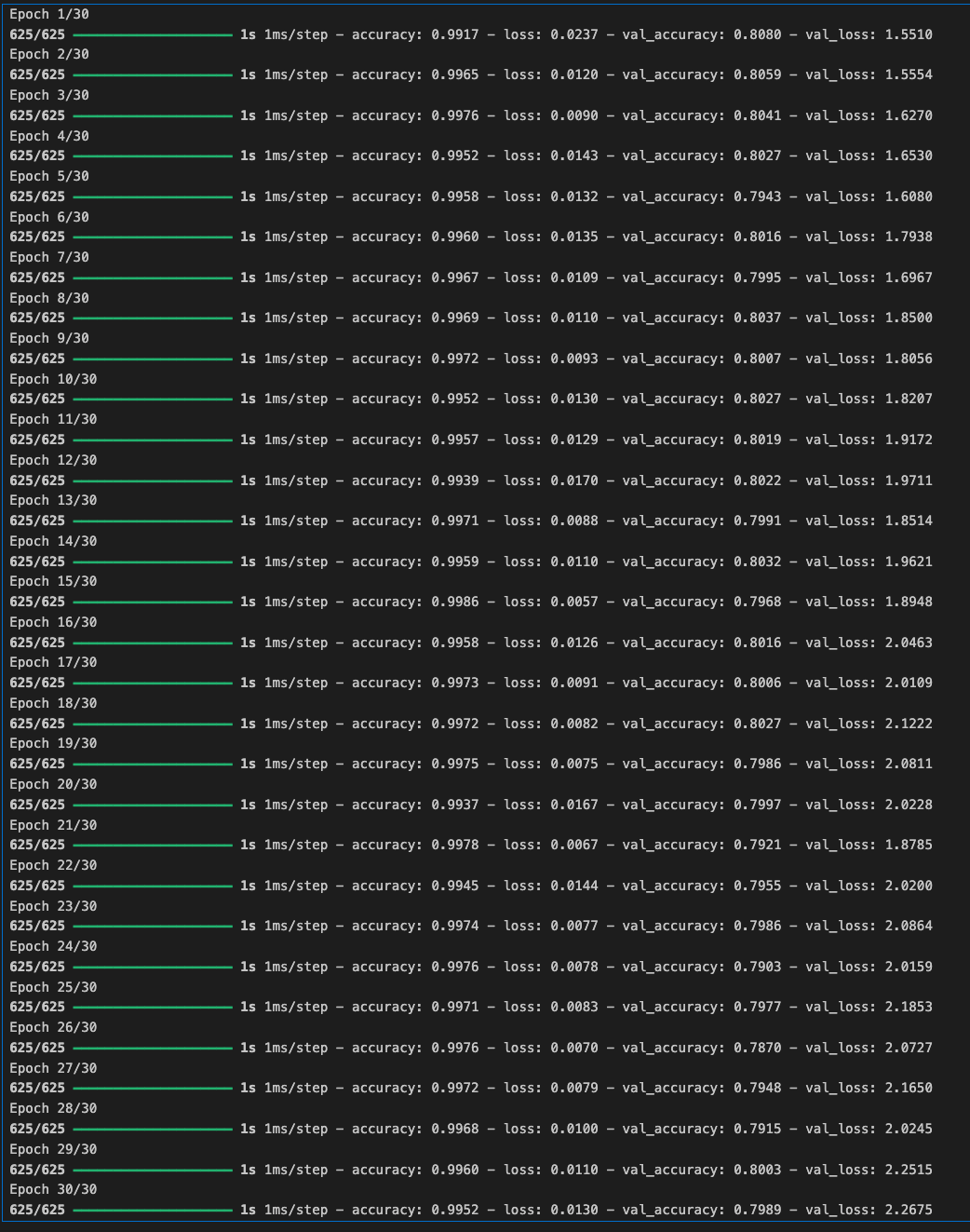

[6] Visualize the Result

• 학습한 모델의 훈련 결과를 플롯해본다.
  훈련 정확도는 계속 올라가는 반면 검증 정확도는 천천히 떨어지기 때문에 약간의 과적합을 발견할 수 있다.
  하이퍼파라미터를 조정하여 이를 개선해본다.

import matplotlib.pyplot as plt

# Plot utility
def plot_graphs(history, string):
  plt.plot(history.history[string])
  plt.plot(history.history['val_'+string])
  plt.xlabel("Epochs")
  plt.ylabel(string)
  plt.legend([string, 'val_'+string])
  plt.show()
  
# Plot the accuracy and loss
plot_graphs(history, "accuracy")
plot_graphs(history, "loss")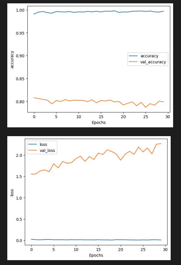

[7] Visualize Word Embeddings

이전과 마찬가지로 Tensorflow Embedding Projector를 사용하여 임베딩의 최종 가중치를 시각화할 수 있다.

https://projector.tensorflow.org/

# Get the index-word dictionary
reverse_word_index = tokenizer.index_word

# Get the embedding layer from the model (i.e. first layer)
embedding_layer = model.layers[0]

# Get the weights of the embedding layer
embedding_weights = embedding_layer.get_weights()[0]

# Print the shape. Expected is (vocab_size, embedding_dim)
print(embedding_weights.shape)

import io

# Open writeable files
out_v = io.open('vecs.tsv', 'w', encoding='utf-8')
out_m = io.open('meta.tsv', 'w', encoding='utf-8')

# Initialize the loop. Start counting at `1` because `0` is just for the padding
for word_num in range(1, vocab_size):

  # Get the word associated at the current index
  word_name = reverse_word_index[word_num]

  # Get the embedding weights associated with the current index
  word_embedding = embedding_weights[word_num]

  # Write the word name
  out_m.write(word_name + "\n")

  # Write the word embedding
  out_v.write('\t'.join([str(x) for x in word_embedding]) + "\n")

# Close the files
out_v.close()
out_m.close()