[Coursera] C1W3 Introduction to TensorFlow , Machine Learning , DeepLearning - Enhancing Vision with Convolutional Neural Networks
DeepLearning.AI TensorFlow Developer

GOAL
- callback function 을 이용하여 accuracy threshold 이후에 훈련 중지
- convolution 과 MaxPoling 을 추가하여 Fashion MNIST classification 정확도 테스트
- convolution 과 MaxPooling 이 image classification 문제에 어떻게 도움을 주는지 설명하고 시각화
Enhancing Vision With Convolutional Neural Networks
L2 What are convolutions and pooling ?
convolution : 이미지의 특징점을 강조할 수 있도록 변형하는 것
pooling : 이미지 압축 방법
Convolution
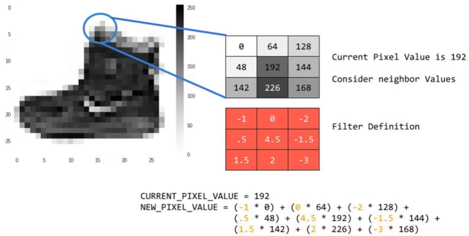
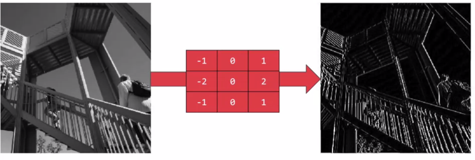
filter 를 이용한 계산으로 이미지의 특징점을 강조
-
vertical feature 강조
-
horizontal feature 강조

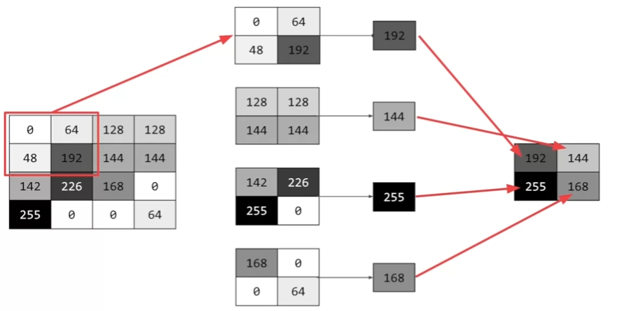
Pooling
이미지 압축 방식 ( 이미지의 특징은 유지된다. )
- 예시 : max pooling
L3 Implementing convolutional layers
이전 코드에 아래 코드를 추가하여 convolutional layer 와 max pooling layer 를 구현할 수 있다.
convolutional layer , max pooling layer 참고 강의 : https://bit.ly/2UGa7uH
model = tf.keras.models.Sequential( [
	tf.keras.layers.Conv2D(64, ( 3,3 ) , activation = 'relu', input_shape = ( 28, 28,1) ),
    tf.keras.layers.MaxPooling2D( 2, 2 ),
    tf.keras.layers.Conv2D( 64, (3,3), activation = 'relu') ,
    tf.keras.layers.MaxPooling2D( 2, 2 ),
    tf.keras.layers.Flatten(),
    tf.keras.layers.Dense( 128, activation='relu'),
    tf.keras.layers.Dense( 10, activation='softmax')
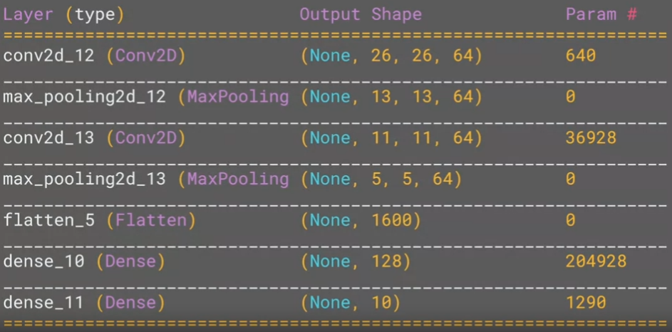
L4 Implementing pooling layers
pooling layer 의 목적 : Convolutional layer 가 결과를 결정하는 데 필요한 특징들만 걸러내도록 하는 것
model.summary()를 이용하면 각 layer 의 parameter 및 단계 별 output shape 을 확인할 수 있다.
참고 : Output shape 계산
- O : Ouput image size
- i : Input image size
- p : padding size
- s : stride
L5 Improving the Fashion classifier with convolutions
convolution : 필터를 통과시켜 이미지 정보량을 줄인다. 이를 통해 신경망이 특징을 효과적으로 학습 할 수 있게 하여 분류 성능을 높임
pooling : 정보를 다루기 쉽도록 압축하여 분류 성능을 높임
DNN 결과
- 5 epoch training loss: 0.2977 - accuracy: 0.8905
- test loss: 0.3368 - accuracy: 0.8809
model = tf.keras.models.Sequential([
	tf.keras.layers.Flatten(),
    tf.keras.layers.Dense( 128, activation = tf.nn.relu ),
    tf.keras.layers.Dense( 10 , activation = tf.nn.softmax )
    ])

    #Setup training parameters
    model.compile( optimizer = 'adam' , loss = 'sparse_categorical_crossentropy',metrics=['accuracy'])

    #Train the model
    print(f'\nMODEL TRAINING:')
    model.fit( training_images , training_labels, epochs=5 )

    # Evaluate on the test set
    print( f'\nMODEL EVALUATION:')
    test_loss = model.evaluate( test_images, test_labels)
Convolution layer 는 3x3 , 5x5 와 같은 필터를 통해 이미지를 스캔한다. 필터와 픽셀 간의 연산을 통해 edge detection 과 같이 특징점을 찾아간다.
Dense layer 에 이미지를 전달하기 전에 convolution 연산을 통해 특징에 더 집중하여 정확도를 높일 수 있도록 한다.
Convolution layer 를 추가한 결과
- 5 epoch training loss: 0.2253 - accuracy: 0.9166
- test loss: 0.2718 - accuracy: 0.9006
model = tf.keras.models.Sequential([
# Add convolutions and max pooling
tf.keras.layers.Conv2D( 32, (3,3) , activation = 'relu' , input_shape = (28,28,1)),
tf.keras.layers.MaxPooling2D(2,2),
tf.keras.layers.Conv2D( 32, (3,3) ,activation = 'relu' ),
tf.keras.layers.MaxPooling2D) 2,2),
# Add the same layers as before
tf.keras.layers.Flatten(),
tf.keras.layers.Dense( 128,activatoin='relu'),
tf.keras.layers.Dense( 10, activation='softmax')
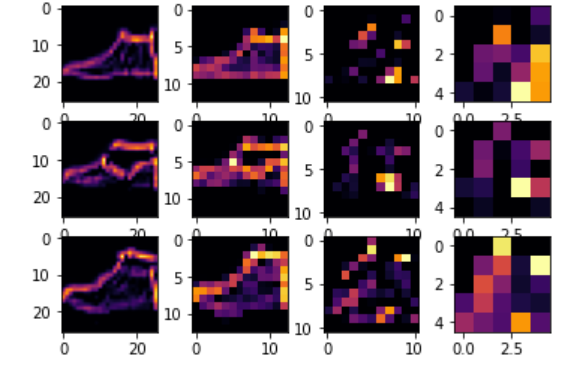
])Visualizing the Convolutions and Pooling
convolution의 과정을 graphic 으로 확인해보자.
Dense layer 이후에는 공통 특징이 발견될 것이다.
import matplotlib.pyplot as plt
from tensorflow.keras import models

f , axarr = plt.subplots( 3,4 )

FIRST_IMAGE = 0
SECOND_IMAGE = 23
THIRD_IMAGE = 28
CONVOLUTON_NUMBER = 3

layer_outputs = [ layer.output for layer in model.layers ]
activation_model = tf.keras.models.Model( inputs = model.input , outputs = layer_outputs )

for x in range( 0,4 ) :
	f1 = activation_model.predict( test_images[FIRST_IMAGE].reshape( 1, 28, 28 ,1 ))[x]
    axarr[0,x].imshow(f1[0,:,:,CONVOLUTION_NUMBER],cmap='inferno')
    axarr[0,x].grid( False )

    f2 = activaiton_model.predict( test_iamges[SECOND_IMAGE].reshape( 1, 28,28, 1))[x]
    axarr[1,x].imshow(f2[0,:,:,CONVOLUTION_NUMBER],cmap='inferno')
    axarr[1,x].grid( False )

    f3 = activatoin_model.predict( test_images[THIRD_IAMGE].reshape(1,28,28,1))[x]
    axarr[2,x].imshow(f3[0,:,:,CONVOLUTION_NUMBER],cmap='inferno')
    axarr[2,x].grid( False )
convolution filter 개수 조절 해보기
-
16개 : 속도는 더 빨랐지만 loss 가 커짐
5 epoch training loss: 0.2591 - accuracy: 0.9055
test loss: 0.2958 - accuracy: 0.8896 -
64개 : 속도는 더 느려졌지만 성능은 개선됨 , 하지만 test set 에서는 큰 차이가 없음
5 epoch training loss: 0.1855 - accuracy: 0.9303
test loss: 0.2729 - accuracy: 0.9024
convolution layer 개수 조절 해보기
-
마지막 레이어 삭제 ( filter 64개 ) : loss 가 줄었음 - filter 개수를 줄여도 비슷한 loss
loss: 0.1464 - accuracy: 0.9458
loss: 0.2554 - accuracy: 0.9120 -
conv layer 2개 , max pooling 1 개 - 가장 좋은 성능
5 epoch training loss : 0.0985 - accuracy: 0.9638
test loss : 0.2683 - accuracy: 0.9200
layer 를 늘렸을 때 성능 저하
- feature 가 과도하게 줄어들면서 소실이 일어났음을 예상할 수 있음
Overfitting
epoch 수를 늘려보면 training accuracy 는 좋아지지만 test accuracy 는 오히려 떨어질 수 있다.
overfitting 문제는 모델의 학습이 training set에 지나치게 맞추어져 , 새로운 데이터 인식률이 낮아지는 것이다.
overfitting 을 방지하는 방법에는 다음과 같은 것들이 있다.
- 데이터 늘리기
- 모델의 복잡도 줄이기
- 가중치 규제 ( Regularization ) 적용하기 : L1 규제 , L2 규제
- Dropout
callback function 작성하기 : training set 정확도가 90% 이상이되면 학습 중지
class myCallback( tf.keras.callbacks.Callback ) :
	def on_epoch_end( self, epoch , logs={}):
    	if logs.get('accuracy')>=0.9 :
        	print("\nReached 90% accuracy so cacelling training! ")
            self.model.stop_training = True
L6 Walking through convolutions
Quiz
-
How do Convolutoins improve image recognition?
answer : They isolate features in images
- convolution layer 는 이미지의 특징점을 강조한다.
-
What does the Pooling technique do to the images ?
answer : Reduces information in them thile maintaining some features
-
How does using Convolutions in our Deep neural network impact training?
answer : It makes it faster
- convolution layer는 이미지의 특징을 강조하고 크기를 줄어 deep neural network 의 속도를 빠르게 해준다.
Week 3: Improve MNIST with Convolutions
GOAL
- model 에 convolution layer 와 max pooling layer 를 추가하여 Fashion MNIST data set 에서 정확도 99.5% 이상을 뽑아보자.
import library
import os
import numpy as np
import tensorflow as tf
from tensorflow import keras
Load the data
# Load the data
# Get current working directory
current_dir = os.getcwd()

# Append data/mnist.npz to the previous path to get the full path
data_path = os.path.join(current_dir, "data/mnist.npz")

# Get only training set
( training_images , training_labels ),_ = tf.keras.datasets.mnist.load(path = data_path)
Pre-processing the data
convolution neural network 에 데이터를 먹이기 전에 정제 ㅈㄱ업이 필요하다.
-
reshape
extra dimension 을 생성하기 위한 reshape
image data 를 표현하기 위해서는 일반적으로 3-dimensional array가 필요하다.
세 번째 dimension 은 RGB 값을 표현한다.
gray scale 을 이용해 흑백으로 표현된 이미지는 세 번째 차원이 필요하지 않지만 좋은 연습이 될거다 ! -
Normalization
pixel 값이 0 과 1 사이에 있도록 nomarization 해준다.