[Coursera] C1W4 Introduction to TensorFlow , Machine Learning , DeepLearning - Using Real-world Images

GOAL

• 이진 분류 모델 구현 시 발견되는 단점에 대한 설명
• Keras ImageDataGenerator functionality 를 활용한 이미지 전처리 실행
• 이진 분류를 위한 multilayer neural network 를 lerveraging 함으로써 현실 이미지 분류 문제 해결
  + 이전에 다루었던 문제는 28x28 size 에 물체가 정중앙에 위치한 것이었지만 , 해당 문제를 다루었던 방법을 확장하여 실세계의 문제에 적용할 수 있다.

Using Real-world Images

L2 Understanding ImageDataGenerator

✔ training set 에서 입력값은 모두 동일한 사이즈여야 한다. - reshape 을 이용하여 일관성 확보

실세계의 이미지들은 물체가 이미지의 정중앙에 위치하지 않은 경우가 더 많으며 크기도 다양하다.
tensorflow의 ImageDataGenerator 를 이용하면 image preprocessing 을 도와준다.

# Import ImageGenerator
from tensorflow.keras.preprocessing.image
import ImageDataGenerator

# instance ImageGenerator and rescale data
train_datagen = ImageDataGenerator( rescale = 1./255 )
train_generator = train_datagen.flow_from_directory(
	train_dir,
    target_size = ( 300 , 300 ) ,
    batch_size = 128 , 
    calss_mode = 'binary' ) 

flow_from_directory

해당 디렉토리 및 하위 디렉토리에서 이미지를 불러온다.

• 하위 디렉토리의 폴더명은 이미지들의 레이블이 됨

 train_datagen.flow_from_directory(
	train_dir,
    target_size = ( 300 , 300 ) ,
    batch_size = 128 , 
    calss_mode = 'binary' ) 

L3 Defining a ConvNet to use complex images

binary classification 문제로 , 0 ~ 1 의 값을 가지는 sigmoid function 사용

( 참고 ) n 개의 labeling 이 필요한 경우 softmax function 을 사용할 수 있지만 , binary classification 문제에서는 sigmoid function 이 조금 더 효율적이다.

convolution layer 가 없었다면 300*300 번의 계산과정이 필요했다.

model = tf.keras.models.Sequential([
	tf.keras.layers.Conv2D( 16 , ( 3,3 ) , activation = 'relu' , input_shape = ( 300,300,3 ) ) ,
    tf.keras.layers.MaxPooling2D( 2,2 ) ,
    tf.keras.layers.Conv2D( 32 , ( 3,3 ) , activation = 'relu'),
    tf.keras.layers.MaxPooling2D( 2,2 ) ,
    tf.keras.layers.Conv2D( 64 , ( 3,3 ) , activation = 'relu'),
    tf.keras.layers.MaxPooling2D( 2,2 ) ,
    tf.keras.layers.Flatten(),
    tf.keras.layers.Dense( 512, activation = 'relu'),
    tf.keras.layers.Dense( 1, activation = 'sigmoid') ])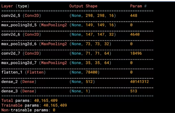

L4 Training the ConvNet

여러 개의 category 를 가지는 Fashion MNIST dataset 을 분류했을 때 , loss function 으로 Categorical Cross Entropy를 사용했다.

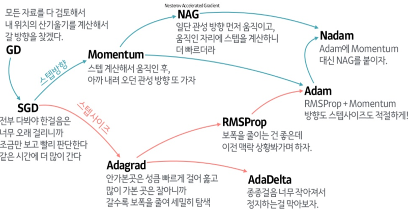
• Adam optimizer 대신 RMSProp 을 사용하여 learning rate 을 실험에 적용시켜보자 !
  

from tensorflow.keras.optimizers import RMSprop

model.compile(loss='binary_crossentropy',
			  optimizer = RMSprop(lr=0.001),
              metrics=['accuracy'])

ImageGenerator 를 사용하기 때문에 model.fit 으로 전달되는 parameters 가 조금 다르다.

history = model.fit(
		train_generator,
        steps_per_epoch=8, # training data set 에는 1024개의 데이터가 있으므로 batch_size 를 128로 하여 8번 불러온다. 
        epochs=15,
        validation_data=validation_generator,
        validation_steps=8,
        verbose=2) # verbose 값에 따라 training 과정을 얼만큼 자세히 보여줄지 결정된다.

학습한 모델을 이용하여 예측해보기

import numpy as np
from google.colab import files
from keras.preprocessing import image

uploaded = files.upload()

for fn in uploaded.keys():
	# predicting images
    path = '/content/' + fn
    img = image.load_img(path, target_size = (300,300)) # input dimension 과 같아야 함 
    x = image.img_to_array(img)
    x = np.expand_dims( x, axis=0)
    
    images = np.vstack([x])
    classes = model.predict(images,batch_size=10)
    print( classes[0])
    if classes[0]>0.5:
    	print(fn+" is a human" )
    else :
    	print(fn+" is a horse" ) 

L5 Walking through developing a ConvNet

Image zip file 압축풀기

import zipfile

# Unzip the dataset
local_zip = './horse-or-human.zip'
zip_ref = zipfile.ZipFile(local_zip , 'r'_
zip_ref.extractall('./horse-or-human')
zip_ref.close()

Image 확인하기

%matplotlib inline

import matplotlib.pyplot as plt
import matplotlib.image as mpimg

# Parameters for our graph; we'll output images in a 4x4 configuration
nrows = 4
ncols = 4

# Index for iterating over images
pic_index = 0 

# Set up matplotlib fig, and size it to fit 4x4 pics
fig = plt.gcf()
fig.set_size_inches(ncols * 4 , nrows * 4)

pic_index += 8
next_horse_pix = [os.path.join(train_horse_dir, fname)
				  for fname in train_horse_names[pic_index-8:pic_index]]
next_human_pix = [os.path.join(train_human_dir, fname) 
				  for fname in train_human_names[pic_index-8:pic_index]]

for i , img_path in enumerate(next_horse_pix , next_human_pix):
	# Set up subplot; subplot indices start at 1
    sp = plt.subplot(nrows, ncols , i+1 ) 
    sp.axis('Off') # Don't show axes ( or gridlines )
    
    img = mpimg.imread(img_path)
    plt.imshow(img)
    
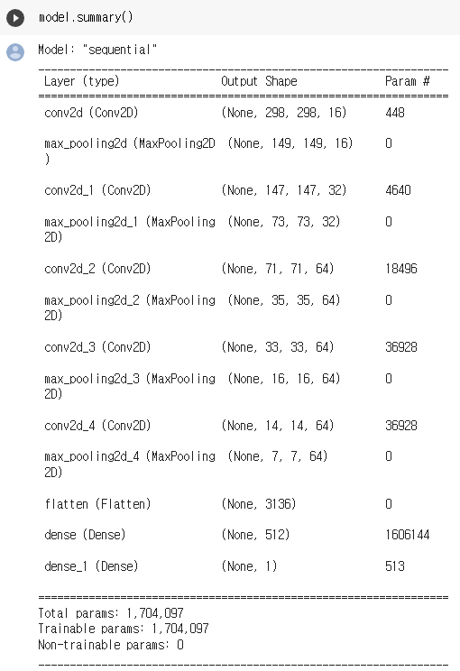
plt.show()

model 구성해보기

• sigmoid function 을 이용하여 horse 와 human 을 분류

model = tf.keras.models.Sequential([
		# Note the input shape is the desired of the image 300x300 with 3 bytes color 
        # This is the first convolution
        tf.keras.layers.Conv2D( 16 , ( 3,3 ) , activation = 'relu' , input_shape=(300,300,3)),
        tf.keras.layers.MaxPooling2D( 2,2 ) ,
        # The second convolution
        tf.keras.layers.Conv2D(32,(3,3),activation='relu'),
        tf.keras.layers.MaxPooling2D(2,2),
        # The third convolution
        tf.keras.layers.Conv2D(64,(3,3),activation='relu'),
        tf.keras.layers.MaxPooling2D(2,2),
        # The fourth convolution
        tf.keras.layers.Conv2D(64,(3,3),activation='relu'),
        tf.keras.layers.MaxPooling2D(2,2),
        # The fifth convolution
        tf.keras.layers.Conv2D(64,(3,3),activation='relu'),
        tf.keras.layers.MaxPooling2D(2,2),
        # Flatten the results to feed into a DNN
        tf.keras.layers.Flatten(),
        # 512 neuron hidden layer
        tf.keras.layers.Dense(512,activiation='relu'),
        tf.keras.layers.Dense(1,activation='sigmoid')
        ])

loss function 과 optimizer 설정하기

SGD 대신 learning rate tune 을 자동으로 해주는 RMSprop 사용 ( Adam , Adagrad 같은 것도 동일한 역할을 함 )

from tensorflow.keras.optimizers import RMSprop

model.compile(loss='binary_crossentropy',
			  optimizer=RMSprop(learning_rate=0.001),
              metrics=['accuracy']
              )

ImageDataGenerator 를 이용하여 Data Preprocessing

folder 안에 있는 이미지들의 preprocessing 을 도와준다.

(참고) 현재는 ImageDataGenerator 대신 tf.keras.utils.image_dataset_from_directory 와 tf.data.Dataset 을 사용할 것을 권장
tensorflow tutorials link : load_image

from tensorflow.keras.preprocessing.image import ImageDataGenerator

# All images will be rescaled by 1./255
train_datagen = ImageDataGenerator(rescale=1/255)

# Flow training images in batches of 128 using train_datagen generator
train_generator = train_datagen.flow_from_directory(
					'./horse-or-human/' , # This is the sourse directory for training images
                    target_size=(300,300),
                    batch_size=128,
                    # Since we use binary_crossentropy loas , we need binary labels
                    class_mode='binary')

L6 Walking through training the ConvNet

Training

• accuracy 변동률을 보면서 learning rate 을 조절할 수 있다.

history = model.fit( train_generator,
  					 steps_per_epoch=8,
                     epochs = 15,
                     verbose = 1 )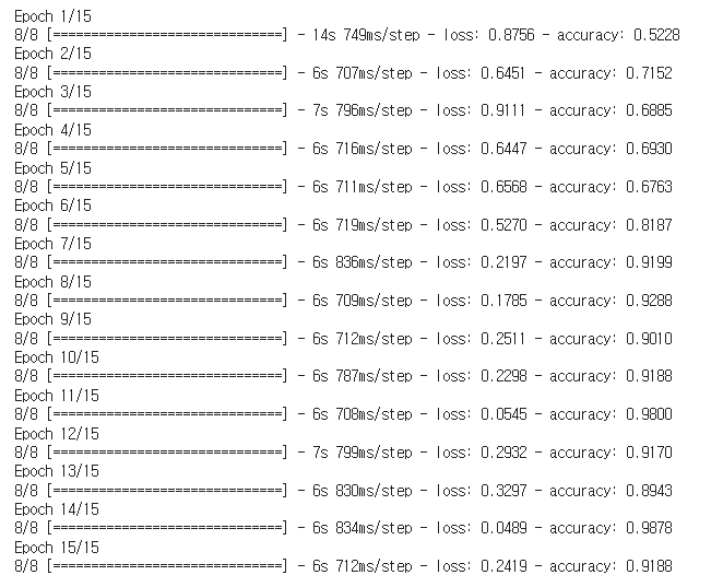 

Model Prediction

import numpy as np
from google.colab import files 
from keras.preprocessing import image

uploaded = files.upload()

for fn in uploaded.keys():

	# predicting images
    path = '/content/' +fn
    img = image.load_img( path, target_size=(300,300))
    x = image.img_to_array(img)
    x /= 255
    x = np.expand_dims(x, axis=0)
    
    images = np.vstack([x])
    classes = model.predict(images,batch_size =10)
    print(classes[0])
    
    if classes[0]>0.5:
       print(fn+" is a human")
    else:
       print(fn+" is a horse")

Visualizing Intermeidate Representations

• feature map 확인하기
  model 을 거치면서 input data 가 어떻게 변화하는지 살펴보자.
• 층이 깊어질수록 추상화 레벨이 높아진다.
• 본래 이미지보다 더 작은 크기의 이미지를 전달하지만 , 특징 정보가 담겨있다.

import numpy as np
import random
from tensorflow.keras.preprocessing.image import img_to_array,load_img

# Define a new Model that will take an image as input, and will output
# intermediate representations for all layers in the previous model after the first.
successive_outputs = [layer.output for layer in model.layer[1:]]
visualization_model = tf.keras.models.Model(inputs=model.input,outputs = successive_ouputs)

# Prepare a random input image from the training set.
horse_img_files = [os.path.join(train_horse_dir,f) for f in train_horse_names]
human_img_files = [os.path.join(train_human_dir,f) for f in train_human_names]
img_path = random.choice(horse_img_files + human_img_files)

img = load_img(img_path, target_size=(300,300)) # this is a PIL image
x = img_to_array(img) # Numpy array with shape (300,300,3)
x = x.reshape((1,)+x.shape) # Numpy array with shape ( 1,300,300,3) 

# Scale by 1/255
x /= 255

# Run the image through the network , thus obtaining all
# intermediate representations for this iamge.
successive_feature_maps = visualization_model.predict(x)

# These are the names of the layers, so you can have them as part of the plot 
layer_names = [layer.name for layer in model.layers[1:]]

# Display the representations
for layer_name, feature_map in zip( layer_names, successive_feature_maps):
	if len(feature_map.shape) == 4 : 
    	# Just do this for the conv / maxpool layers , not the fully-connected layers 
        n_features  = feature_map.shape[-1] # number of features in feature map 
        size = feature_map.shape[1]
        
        # Tile the images in the matrix
        display_grid = np.zeros((size, size * n_features))
        for i in range(n_features):
        	x  = feature_map[0,:,:,i]
            x -= x.mean()
            x /= x.std()
            x *= 64
            x += 128
            x = np.clip( x,0,255).astype('uint8')
            
            # Tile each filter into this big horizontal grid
            display_grid[:,i*size:(i+1)*size] = x
            
        # Display the grid
        scale = 20. / n_features
        plt.figure(figsize=(scale * n_features, scale))
        plt.title(layer_name)
        plt.grid(False)
        plt.imshow(display_grid,aspect='auto', camp='viridis')

메모리 정리

import os, signal
os.kill(os.getpid(), signal.SIGKILL)

L7 Adding automatic validation to test accuracy

• training loop 에 validation 체계를 구축하고 ,tensorflow 를 이용하여 검증 효과를 측정

• 테스트를 통해 훈련 데이터 셋의 문제를 추측해볼 수 있음

• 하얀 말 사진이 많구나 ..! <- 하얀 말만 잘 인식함

• 전신 사진이 많구나 ..! <- 반신 사진은 인식하지 못함

Validation dataset 추가

import os

# Directory with training horse pictures
train_horse_dir = os.path.join('./horse-or-human/horses')

# Directory with training human pictures
train_human_dir = os.path.join('./horse-or-human/humans')

# Directory with validation horse pictures
validation_horse_dir = os.path.join('./validation-horse-or-human/horses')

# Directory with validation human pictures
validation_human_dir = os.path.join('./validation-horse-or-human/humans')

Validation Generator 추가

from tensorflow.keras.preprocessing.image import ImageDataGenerator

# All images will be rescaled by 1./255
train_datagen = ImageDataGenerator(rescale=1/255)
validation_datagen = ImageDataGenerator(rescale=1/255)

# Flow training images in batches of 128 using train_datagen generator
train_generator = train_datagen.flow_from_directory(
        './horse-or-human/',  # This is the source directory for training images
        target_size=(300, 300),  # All images will be resized to 300x300
        batch_size=128,
        # Since you use binary_crossentropy loss, you need binary labels
        class_mode='binary')

# Flow validation images in batches of 128 using validation_datagen generator
validation_generator = validation_datagen.flow_from_directory(
        './validation-horse-or-human/',  # This is the source directory for validation images
        target_size=(300, 300),  # All images will be resized to 300x300
        batch_size=32,
        # Since you use binary_crossentropy loss, you need binary labels
        class_mode='binary')

model 학습 시에 validatoin data 전달

history = model.fit(
      train_generator,
      steps_per_epoch=8,  
      epochs=15,
      verbose=1,
      validation_data = validation_generator,
      validation_steps=8)

L7 Exploring the impact of compressing images

image size 를 150x150 으로 줄여서 테스트 결과

• 빠른 학습 속도
• 과적합 가능성 ( training set 의 accuracy 가 0.99 로 지나치게 높게 나옴 )
• 정확도가 떨어짐

Quiz

3. How did we specify the training size for the images?

   The target_size parameter on the training generator

4. Convolutional Neural Networks are better for classifying images like horses and humans because:

• There’s a wide variety of horses
• In these images, the features may be in different parts of the frame
• There’s a wide variety of humans

7. After reducing the size of the images, the training results were different. Why?

   We removed some convolutions to handle the smaller images.

Week 4: Handling Complex Images - Happy or Sad Dataset

80 개의 happy / sad image data set 을 이용해보자.
이 이미지에 대해 99.9% 의 정확도를 가지는 모델을 만들고 , threshold 이상으로 정확도가 높아지면 트레이닝을 중단해보자.

library import

import matplotlib.pyplot as plt
import tensorflow as tf
import numpy as np
import os

Load and explore the data

image 들은 data 라는 상위 폴더 밑에 happy 와 sad 로 분류되어 들어있다.

from tensorflow.keras.preprocessing.image import load_img

base_dir = "./data/"
happy_dir = os.path.join( base_dir , "happy/")
sad_dir = os.path.join( base_dir , "sad/")

print("Sample happy image:")
plt.imshow(load_img(f"{os.path.join(happy_dir, os.listdir(happy_dir)[0])}"))
plt.show()

print("\nSample sad image:")
plt.imshow(load_img(f"{os.path.join(sad_dir,os.listdir(sad_dir)[0])}"))
plt.show()

sample image 확인 해보기

• network 첫 번째 layer의 input size 는 input image resolution 과 동일해야한다.

from tensorflow.keras.preprocessing.image import img_to_array

# Load the first example of a happy face
sample_iamge = load_img(f"{os.path.join(happy_dir,os.listdir(happy_dir)[0])}")

# Convert the image into its numpy array representation
sample_array = img_to_array(sample_image)

print(f"Each image has shape: {sample_array.shape}")

print(f"The maximum pixel value used is : {np.max(sampe_array)}")

# Each image has shape: (150, 150, 3)
# The maximum pixel value used is: 255.0

Defining the callback

(참고) 우리는 on_epoch_end function 만 사용했지만 , EarlyStopping callback 을 정의하면 model 에서 가장 좋은 성능을 낸 weights 를 저장할 수도 있다.

class myCallback( tf.keras.callbacks.Callback):
	def on_each_end(self, epoch,logs={}):
    	if logs.get('accuracy') is not None and logs.get('accuracy') > 0.999:
        	print("\nReached 99.9% accuracy so cancelling training!")
            self.model.stop_training = True

Pre-processing the data

• directory : image 가 저장되어 있는 directory 의 상대 경로
• target_size : color dimension 을 제외하고 image 의 resolution 과 동일하게 설정
• batch_size : 한 번에 처리할 데이터 양
• class mode : label을 표현할 방법 - binary , categorical ,sparse

from tensorflow.keras.preprocessing.image import ImageDataGenerator

def iamge_generator():
	# ImageDataGenerator class 를 생성할 때 , rescale parameter를 전달해준다. 
	train_datagen = ImageDataGenerator( rescale = 1./255 )
    
    train_generator = train_datagen.flow_from_directory( directory = './data/',
    													 target_size = (150,150),
                                                         batch_size = 10 ,
                                                         class_mode = 'binary') 
 return train_generator
 
 # Save your generator in a variable
 gen = image_generator()

Creating and training your model

from tensorflow.keras import optimizers, losss

def train_happy_sad_model(train_generator):
	callbacks = myCallback()
    
    # Define the model
    model = tf.keras.models.Sequential([
        tf.keras.layers.Conv2D(16,(3,3),activation='relu',input_shape=(150,150,3)) ,
        tf.keras.layers.MaxPooling2D(2,2),
        tf.keras.layers.Conv2D(32,(3,3), activation = 'relu'),
        tf.keras.layers.MaxPooling2D(2,2),
        tf.keras.layers.Conv2D(64,(3,3), activation = 'relu'),
        tf.keras.layers.MaxPooling2D(2,2),
        tf.keras.layers.Flatten(),
        tf.keras.layers.Dense(512, activation='relu'),
        tf.keras.layers.Dense(1 , activation='sigmoid')

    ])

    # Compile the model
    # Select a loss function compatible with the last layer of your network
    model.compile(loss=losses.binary_crossentropy,
                  optimizer=optimizers.Adam(learning_rate=0.001),
                  metrics=['accuracy']) 
    


    # Train the model
    # Your model should achieve the desired accuracy in less than 15 epochs.
    # You can hardcode up to 20 epochs in the function below but the callback should trigger before 15.
    history = model.fit(x=train_generator,
                        epochs=15,
                        callbacks=[callbacks]
                       ) 
    
    ### END CODE HERE
    return history
    
hist = train_happy_sad_model(gen)