[Coursera] C2W3 Convolutional Neural Networks in TensorFlow - Augmentation: Transfer Learning

GOAL

• overfitting 을 피하기 위한 dropout 효과를 주는 keras layer type 을 마스터 해보자 !
• keras API 를 통해 transfer learning 을 해보자.
• Sequential mdoel 대신 keras functional API 로 모델을 코딩해보자.
• 성공적인 transfer learning 을 구현하기 위해 존재하는 모델로 부터 later 를 freeze 하는 방법을 알아보자.
• 대형 dataset으로 부터 학습된 다른 모델의 convolutions 를 사용하기 위한 transfer learning 개념 학습

L2 : Understanding transfer learning: the concepts

훨씬 많은 데이터로 학습된 모델을 활용하는 방법 : transfer learning

• 학습 레이어를 고정시키고 모델이 학습한 컨볼루션을 이용하여 Dense layer 만 새롭게 학습시켜 사용하는 방법
• 학습 레이어의 일부를 새롭게 학습시켜 모델의 fit 을 높일 수 있다.

( 실습 ) 140만개의 데이터 셋을 1,000개의 class 로 분류하는 imagenet의 dataset 으로 훈련된 inception 모델을 이용해 transfer learning 을 배워보자

• imagenet

L3 Coding transfer learning from the inception model

library import

import os 
from tensorflow.keras import layers
from tensorflow.keras import Model

아래 링크에서 사전에 훈련해둔 가중치의 사본을 다운받을 수 있다.

• inception neural network : 현재 동작 x

Inception 사용하기

keras 에는 inception_v3 모델이 내재되어 있다.
기존에 학습된 가중치를 이용하여 모델을 학습시켜 보자.

• include_top : inception_v3 상단에 있는 fully connected layer 를 사용할지에 대한 여부

from tensorflow.keras.applications.inception_v3 import InceptionV3

local_wights_file = 'tmp/inception_v3_weights_tf_dim_ordering_tf_kernels_notop.h5'

pre_trained_model = InceptionV3(input_shape = 					  ( 150,150,3 ),
					include_top = False ,  
					weights = None )

layer 비활성화 : 모델을 재사용하기 위함

for layer in pre_trained_model.layers:
    layer.trainable = False

pre_trained_model.summary()

Adding your DNN

Now, you'll need to add your own DNN at the bottom of these, which you can retrain to your data.

L4 Coding your own model with transferred features

pre-trained model 에 DNN 을 추가하여 학습하고자 하는 dataset 에 대한 분류 모델로 사용할 수 있다.

layer 이름으로 output value 가져오기

last_layer = pre_trained_model.get_layer('mixed7')
last_output = last_layer.output

DNN 추가하기

from tensorflow.keras.optimizers import RMSprop

x = layers.Flatten()(last_output)
x = layers.Dense( 1024, activation = 'relu')(x)
x = layers.Dense( 1 , activation = 'sigmoid')(x)

model = Model( pre_trained_model.input , x ) 
model.compile( optimizer = RMSprop(learning_rate = 0.0001 ),
			   loss = 'binary_crossentropy',
			   metrics = ['acc'])

ImageDataGenerator 로 input data 준비

# Add our data-augmentation parameters to ImageDataGenerator

train_datagen = ImageDataGenerator( rescale = 1./255.,
								    rotation_range = 40,
								    width_shift_range = 0.2 , 
								    height_shift_range = 0.2 ,
								    shear_range = 0.2 , 
								    zoom_range = 0.2 , 
								    horizontal_flip = True )

flow_from_directory 로 데이터 얻기

train_generator = train_datagen.flow_from_directory( train_dir, 
				  batch_size = 20 , 
				  class_mode = 'binary',
				  target_size = (150,150))

모델 학습시키기

history = model.fit( 
			train_generator , 
            validation_data = validation_generator , 
            steps_per_epoch = 100,
            epochs = 100,
            validation_steps = 50,
            verbose = 2 ) 

과적합 양상 분석

• validation accuracy 가 발산하면서 줄어드는 모양새

  이런 형태의 overfitting 을 방지하기 위해서는 어떻게 해야할까 ? :

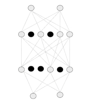
  • dropout : to remove a random number of neurons in your neural network
  • dropout 이 overfitting 방지에 효과적인 이유
    - 인접한 neuron들은 비슷한 weight 를 가져 overfitting 을 야기한다. random drop out 을 이용하면 해당 부분을 방지할 수 있다.
    - neuron 은 이전 layer의 neuron 의 input 을 over-weight 하는 경향이 있어 overfitting 을 야기한다.

L5 Exploring dropouts

dropout : neural network 에서 random 으로 몇몇 neuron 을 제거하는 것

• 인접한 neuron 들이 서로 영향을 주지 못하게 연결고리를 끊는다. → overfitting 방지 효과

dropout code 작성하기

• 20% 의 확률로 dropout 하는 코드

x = layers.Dropout(0.2)(x)

from tensorflow.keras.optimizers import RMSprop

x = layers.Flatten()(last_output)
x = layers.Dense( 1024, activation='relu')(x)
x = layers.Dropout(0.2)(x) # 20%의 확률로 dropout
x = layers.Dense( 1 , activation = 'sigmoid')(x)

model = Model( pre_trained_model.input , x ) 
model.compile( optimizer = RMSprop(lr = 0.001) , 
			   loss = 'binary_crossentropy',
			   metrics = ['acc'])

시간이 지날수록 validation accuracy 가 낮아지면서 diversing 하면 dropout 사용을 고려해보자. !

( 참고 ) tensorflow transfer_learning 공식문서 바로가기

L6 Exploring Transfer Learning with Inception

C2_W3_Lab_1_transfer_learning 코드 보기

Transfer learning

• model 에서 convolution layer 가져오기
• dense layer 붙이기
• dense layer 학습하기
• 결과 평가

Pretrained model 설정하기

( 참고 ) 예시 basemodel : InceptionV3

• 내 application 에 맞는 input shape 설정하기
• output으로 사용할 것과 freeze 할 convolution layer 고르기 ( 이전 학습으로 부터 이점이 될만한 방향으로 생각해서 고르자 )
• train 시킬 dense layer 추가하기

pretrained model 가져오기

from tensorflow.keras.applications.inception_v3 import InceptionV3
from tensorflow.keras import layers

# Set the weights file you downloaded into a variable
local_weights_file = '/tmp/inception_v3_weights_tf_dim_ordering_tf_kernels_notop.h5'

# Initialize the base model.
# Set the input shape and remove the dense layers
pre_trained_model = InceptionV3( input_shape = ( 150,150,3),
								 include_top = False , 
								 weights = None ) 
                                 
# Load the pre-trained weights you downloaded 
pre_trained_model.load_weights(local_weights_filie) 

# Freeze the weights of the layers.
for layer in pre_trained_model.layers
	layer.trainable = False 

pretrained model summary 확인

pre_trained_model.summary()

• Inceptionnet_V3는 아주 깊은 모델이다.
• layer 가 깊어질수록 특정 데이터에 specialize 되기 때문에 , 강의에서는 mixed_7 layer 의 output value 를 사용한다.
• ( todo ) output value 를 가져올 layer 의 이름을 바꾸면서 실험해보자 ! `

mixed_7 layer 확인

# Choose 'mixed_7' as the last layer of your base model 
last_layer = pre_trained_model.get_layer('mixed7')
print('last layer output shape : ' , last_layer.output_shape)
last_output = last_layer.output

Dataset 에 맞는 분류를 위해 Dense layer 추가하기

• overfitting 을 피하기 위해 dropout 도 적용해보자.

from tensorflow.keras.optimizers import RMSprop
from tensorflow.keras import Model

# Flatten the output layer to 1 dimension
x = layers.Flatten()(last_output)
# Add a fully connected layer with 1,024 hidden units and ReLU activation
x = layers.Dense(1024,activation='relu')(x)
# Add a dropout rate of 0.2
x = layers.Dropout(0.2)(x)
# Add a final sigmoid layer for classificatoin
x = layers.Dense( 1, activation = 'sigmoid')(x)

# Append the dense network to the base model
model = Model(pre_trained_model.input,x)

# Print the model summary. See your dense network connected at the end.
model.summary()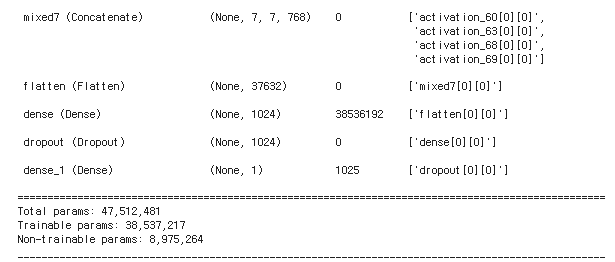

model compile 하기

# Set the training parameters
model.compile( optimizer = RMSprop( learning_rate = 0.0001) , 
loss = 'binary_crossentropy',
metrics = ['accuracy'])

dataset 준비하기

ImageDataGenerator 를 이용하여 데이터를 준비해보자.

• test_datagen 은 augmentation 을 적용하지 않음에 주의

import os
import zipfile
from tensorflow.keras.preprocessing.image import ImageDataGenerator

# Extract the archive
zip_ref = zipfile.ZipFile("./cats_and_dogs_filtered.zip", 'r')
zip_ref.extractall("tmp/")
zip_ref.close()

# Define our example directories and files 
base_dir = 'tmp/cats_and_dogs_filtered'

train_dir = os.path.join( base_dir , 'train' ) 
validation_dir = os.path.join( base_dir , 'validation' ) 

# Directory with training cat pictures
train_cats_dir = os.path.join(train_dir , 'cats')

# Directory with training dog pictures
train_dogs_dir = os.path.join(train_dir,'dogs')

# Directory with validation cat pictures
validation_cats_dir = os.path.join( validation_dir , 'cats')

# Directory with validation dog pictures
validation_dogs_dir = os.path.join( validation_dir , 'dogs' )

# Add our data-augmentation parameters to ImageDataGenerator
train_datagen = ImageDataGenerator( rescale = 1./255.,
				rotation_range = 40,
				width_shift_range = 0.2, 
				height_shift_range = 0.2,
				shear_range = 0.2, 
				zoom_range = 0.2,
				horizontal_flip = True )

# Note that the validation data should not be augmented! 
test_datagen = ImageDataGenerator( rescale = 1.0/255. ) 

# Flow training images in batches of 20 using train_datagen generator
train_generator = train_datagen.flow_form_directory( train_dir , 
				  batch_size = 20,
				  class_mode = 'binary',
				  target_size = ( 150,150) ) 

# Flow validation images in batches of 20 using test_datagen generator
validation_generator = test_datagen.flow_from_directory( validation_dir, 
					   batch_size = 20 , 
					   class_mode = 'binary',
					   target_size = ( 150,150)) 

Train the model

20 epochs 학습하고 plot 그려보기

# Train the model.
history = model.fit(
		  train_generator,
          validation_data = validation_generator,
          steps_per_epoch = 100, # 20*100 = 2,000
          epochs = 20,
          validation_steps = 50 , 
          verbose = 2 ) 

Evaluation the resluts

training accuracy 와 validation accuracy 를 그래프로 그려보자.

• validation accuracy 가 training accuracy 를 추종하는 면이 있다. This is a good sign that your model is no longer overfitting!

import matplotlib.pyplot as plt
acc = history.history['accuracy']
val_acc = history.history['val_accuracy']
loss = history.history['loss']
val_loss = history.history['val_loss']

epochs = range(len(acc))

plt.plot(epochs , acc , 'r', label = 'Training accuracy')
plt.plot(epochs , val_acc , 'b' , label = 'Validation accuarcy')
plt.title('Training and Validation accuracy')
plt.legend(loc = 0 ) 
plt.figure()

plt.show()

Quiz

3. How did you lock or freeze a layer from retraining?

   layer.trainable = false

4. Why do dropouts help avoid overfitting?

   Because neighbor neurons can have similar weights, and thus can skew the final training

Assignment : Week 3: Transfer Learning

Week 3: Transfer Learning 코드 바로가기
Transfer learning 기존에 학습된 모델에 DNN 을 추가하여 가지고 있는 dataset 에 맞는 분류 모델을 생성하는 것

• overfitting 이 발생했을 때는 dropout을 생각해보자.