[Coursera] C3W3 Neural Language Processing in TensorFlow - Sequence models

윰진·2022년 9월 12일

DeepLearning.AI TensorFlow Developer

목록 보기

11/12

GOAL

2주차에는 Embedding layer 를 통해 유사한 단어를 그룹짓는 일을 했다.

이번 주차에는 맥락 속에서 단어의 관계를 파악해보자 !

L2 Introduction

코세라 - 앤드류의 Deep RNN 강의 바로가기

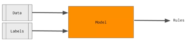
Model 은 data 와 label 을 통해 rule 를 찾아낸다.
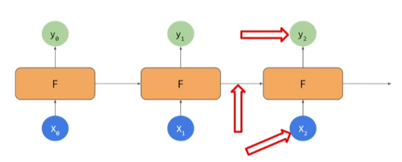
Recurrent Nueural Network 는 이전 인풋에서 도출된 아웃풋을 이용하여 다음 아웃풋을 산출한다.

L3 LSTMs ( Long Short Turm Memorys )

코세라 - 앤드류의 LSTM 강의 바로가기

언어는 단어와 맥락을 통해 유추할 수 있다.
- 아래 문장에서는 blue 가 key 가 되어 sky 를 유추할 수 있다.
때로는 앞선 단어가 key 값이 되는 경우도 있다. 이 때 사용되는 것이 LSTMs 이다.

L4 Implementing LSTMs in code

Bidirectional layer 로 감싸면 Both direction 으로 만든다.

model = tf.keras.Sequenctial([
    tf.keras.layers.Embedding(tokenizer.vocab_size , 64 ) , 
  # tf.keras.layers.Bidirectional(tf.keras.layers.LSTM(64, return_sequences = True ) ),
  # tf.keras.layers.Bidirectional(tf.keras.layers.LSTM(32)), tf.keras.layers.Bidirectional(tf.keras.layers.LSTM(64)),
    tf.keras.Dense(64,activation = 'relu'),
    tf.keras.layers.Dense(1,activation='sigmoid')

C3_W3_Lab_1_single_layer_LSTM.ipynb 코드 바로가기

앞선 과제에서 우리는 기본 dense layer 와 embedding layer 를 이용하여 단어의 결합으로 분류를 결정했다. 이번 노트북에서는 Recurrent Neural Networks 같은 기본 모델을 다룰 것이다. 이 모델은 인풋의 순서를 받아들여 다룬다.
1: My friends do like the movie but I don't. --> negative review
2: My friends don't like the movie but I do. --> positive review
첫 번째 레이어로는 LSTM (Long Short-Term Memory) 을 살펴본다. 이 레이거는 현재 timestamp 와 과거의 timesteps 를 계산하여 상태를 업데이트한다. 이 과정은 이전 모든 단계에서 영향을 받은 output computation 이 있는 마지막 timestep 까지 반복된다. 뿐만 아니라, bidirection 으로 영향을 줄 수 있어 , 나중 단어와 앞선 단어의 관계를 얻을 수 있다. 이 과정이 어떻게 동작하는지 알고 싶으면 Sequence Models 이 강좌를 듣자. 이번 랩에서는 TF API의 이점을 알아보자.

데이터셋 로드하기

이번 랩에서는 IMDB Reviews dataset 이 미리 tokenized 된 subwords8k 를 사용한다. Tensorflow 를 통해 load 할 수 있다.

import tensorflow_datasets as tfds

# Download the subword encoded pretokenized dataset
dataset , info = tfds.load('imdb_reviews/subwords8k', with_info=True , as_supervised = True ) 

# Get the tokenizer
tokenizer = info.features['text'].encoder

데이터셋 준비하기

train 과 test 로 분리된 dataset 과 padded batches 를 얻을 수 있다.
Note : training 을 빠르게 만들기 위해 로렌스가 했던 것 처럼 batch size 를 늘릴 수 있다. 특히 batch size 로 256 을 사용할 수 있고 이 때 한 에포크 당 훈련시간이 거의 1분 걸린다. 이 영상에서 로렌스는 batch size 로 16을 사용했고 에포크 당 4분이 걸렸다.

BUFFER_SIZE = 10000
BATCH_SIZE = 256

# Get the train and test splits
train_data , test_data = dataset['train'], dataset['test'],

# Shuffle the training data
train_dataset = train_data.shuffle(BUFFER_SIZE) 

# Batch and pad the datasets to the maximu length of the sequences
train_dataset = train_dataset.padded_batch(BATCH_SIZE)
test_dataset = test_data.padded_batch(BATCH_SIZE)

모델 구성하고 컴파일 하기

이제 모델을 구성해보자. LSTM layer 전에 등장하는 Flatten() 과 GlobalAveragePooling1D 는 서로 바꿔가며 테스트 할 수 있다. 더 나아가, 앞 뒤로 값을 전달하기 위해 Biderectional layer 안에서 중첩시킬 수 있다. 이런 추가 계산은 훈련속도를 늦출 수 있기 때문에 , 실제 애플리케이션에 RNN 을 적용할 때 고려해야 한다.

import tensorflow as tf

# Hyperparameters
embedding_dim = 64
lstm_dim = 64
dense_dim = 64

# Build the model
model = tf.keras.Sequential([
    tf.keras.layers.Embedding(tokenizer.vocab_size , embedding_dim),
    tf.keras.layers.Bidirectional(tf.keras.layers.LSTM(lstm_dim)),
    tf.keras.layers.Dense(dense_dim , activation = 'relu'),
    tf.keras.layers.Dense( 1, activation = 'sigmoid')
    ])
    
 # Print the model summary
 model.summary()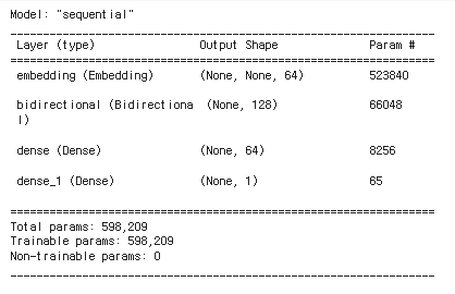

# Set the training parameters
model.compile(loss='binary_crossentropy', optimizer='adam', metrics=['accuracy'])

모델 훈련시키기

default 값을 그대로 가져가면 98% 의 훈련 정확도와 82% 의 validation 정확도를 얻을 수 있다. plot 화하여 확인해보고 , epoch 수를 늘리거나 hyperparameter 를 수정했을 때 어떤 일이 생기는지 확인해보자.

NUM_EPOCHS = 10
history = model.fit(train_dataset, epochs=NUM_EPOCHS , validation_data = test_dataset)

그래프 그리기

import matplotlib.pyplot as plt 

# Plot utility 
def plot_graphs(history , string):
    plt.plot(history.history[string])
        plt.plot(history.history['val_'+string])
        plt.xlabel("Epochs")
        plt.ylabel(string)
        plt.legend?([string, 'val_'+string])
        plt.show()
        
# Plot the accuracy and results
plot_graphs( history , "accuracy")
plot_graphs( history , "loss")

이로써 Recurrent Neural Networks를 구축하기 위해 LSTM layer 를 사용해봤다. 이번에는 하나의 layer 만 사용했지만 , 더 깊은 네트워크를 쌓을 수 있다. 다음 lab 에서 알아보자.

C3_W3_Lab_2_multiple_layer_LSTM.ipynb 코드 바로가기

multiple LSTM layers 에 대해 알아보자.

Lab1 에서 앞부분을 다루었으니 이번에는 모델에 집중해보자.

Build and Compile the Model

-Sequence model 에 LSTM layer 를 추가하여 multiple layer LSTM model 을 구성할 수 있다. LSTM layer 는 input 으로 sequences 를 기대하기 때문에, return_sequences 값을 True 로 주어 output 값을 sequences 로 받을 수 있다. return_sequences 값이 True 일 때 , output이 3차원 (batch_size, timesteps, features) 임을 알 수 있다.

이 값에 따라 마지막 시퀀스에서 한 번만 출력할지 , 각 시퀀스에서 출력할지 결정된다. 참고_김태영님의 순환 신경망 레이어 이야기
return_sequences 값에 따른 결과 테스트

import tensorflow as tf
import numpy as np

# Hyperparameters
batch_size = 1
timesteps = 20
features = 16
lstm_dim = 8

print(f'batch_size: {batch_size}')
print(f'timesteps ( sequence length ) : { timesteps }')
print(f'features ( embedding size ) : { features }')
print(f'lstm output units : {lstm_dim}')

# Define array input with random values 
random_input = np.random.rand(batch_size , timesteps , features ) 
print( f 'shape of input array : { random_input.shape }')

# Define LSTM that returns a single output 
lstm = tf.keras.layers.LSTM(lstm_dim)
result = lstm( random_input)
print(f'shape of lstm output(return_sequences=False): {result.shape}')

# Define LSTM that returns a sequence
lstm_rs = tf.keras.layers.LSTM(lstm_dim, return_sequences = True )
result = lstm_rs(random_input)
print(f'shape of lstm output(return_sequences = True ) : {result.shape}')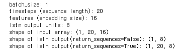

LSTM architecure 쌓기

import tensorflow as tf

# Hyperparameters
embedding_dim = 64
lstm1_dim = 64
lstm2_dim = 32
dense_dim = 64

# Build the model
model = tf.keras.Sequenctial([
    tf.keras.layers.Embedding(tokenizer.vocab_size , embedding_dim),
    tf.keras.layers.Bidirectional(tf.keras.layers.LSTM(lstm1_dim , return_sequences = True)),
    tf.keras.layers.Bidirectional(tf.keras.layers.LSTM(lstm2_dim)),
    tf.keras.layres.Dense(dense_dim , activation='relu'),
    tf.keras.layers.Dense(1,activation='sigmoid')
    ])
    
# Print the model summary
model.summary()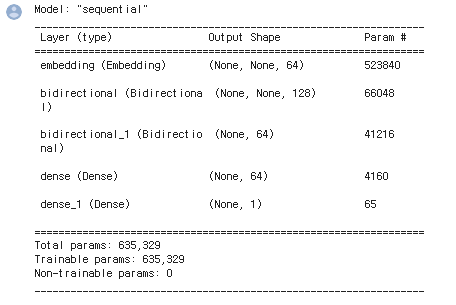

# Set the training parameters
model.compile(loss='binary_crossentropy', optimizer = 'adam', metrics = ['accuracy'])

Train the Model

LSTM layer 가 추가됨에 따라 학습시간이 길어졌다. 주어진 default parameters 그리고 Colab GPU 환경에서 한 에포크당 약 2분정도의 시간이 걸린다.

시각화

import matplotlib.pyplot as plt

# Plot utility
def plot_graphs( history, string):
    plt.plot( history.history[string])
    plt.plot(history.history['val_' + stirng ] )
    plt.xlabel("Epochs")
    plt.ylabel(string)
    plt.legend([string , 'val_'+string])
    plt.show()
    
# Plot the accuracy and results
plot_graphs(history , "accuracy")
plot_graphs(history , "loss")

L5 Accuracy and loss

single LSTM 과 multiple LSTM 의 accuracy 그래프는 큰 차이가 없다.
train accuracy 곡선이 multiple LSTM 에서 부드러워진 것을 볼 수 있다.
train accuracy 가 들쑥날쑥한 것은 모델 개선의 신호가 된다.

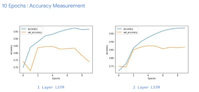
epoch 를 늘려보면 single LSTM 이 보여주는 변동성이 모델 전체 성능에 대한 의구심이 들게 할 수 있다.
반면 multiple LSTM 모델에서는 비교적 부드러는 그래프를 볼 수 있다.

C3_W3_Lab_3_Conv1D.ipynb 코드 바로가기

Convolution layer 활용해보기

Build the Model

이미지 데이터를 다룰 때는 Conv2D layer 를 사용했다. 하지만 , text sequences 처럼 temporal data 를 다룰 때는 Conv1D 를 사용하여 convolution 이 single dimension 에서 동작하게 한다. 이 때 , convolutional layer 의 output 을 줄이기 위해 pooling layer 를 함께 추가할 수 있다. 이번 랩에서는 time dimesion 에 걸쳐 가장 큰 값을 얻는 GlobalMaxPooling1D 를 사용할 것이다. Average pooling 을 사용할 수 도 있는데 , 이건 다음 랩에서 진행한다.

Conv1D 와 GlobalMaxPooling1D layer 의 동작 방식 알아보기

# Pass array to convolution layer and inspect output shape 
conv1d = tf.keras.Conv1D( filters=filters, kernel_size = kernel_size , activation = 'relu')
result = conv1d(random_input)
print(f'shape of conv1d output: {result.shape}')

# Pass array to max pooling layer and inspect output shape
gmp = tf.keras.layers.GlobalMaxPooling1D()
result = gmp(result)
print(f'shape of global max pooling output : {reusult.shape}')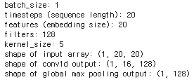

모델 구성해보기

import tensorflow as tf

# Hyperparameters
embedding_dim = 64
filters = 128
kernel_size = 5 
dense_dim = 64

# Build the model
model = tf.keras.Sequential([
    tf.keras.layers.Embedding(tokenizer.vocab_size , embedding_dim),
    tf.keras.layers.Conv1D(filters=filters, kernel_size = kernel_size , activation='relu'),
    tf.keras.layers.GlobalMaxPooling1D(),
    tf.keras.layers.Dense(dense_dim, activation='relu'),
    tf.keras.layers.Dense(1, activation='sigmoid')])
    

# Print the model summary
model.summary()

Train the model

한 에포크당 30초 정도의 훈련시간이 걸리며 , 이전 모델보다 정확도가 향상됨

NUM_EPOCHS = 10 

# Train the model 
history = model.fit(train_dataset, epochs = NUM_EPOCHS , validation_data = test_data)

L7 Looking into the code

LSTM model 을 사용하면 초반부터 꽤 높은 accuracy 를 보여준다.
이후 점점 줄어들지만, 그래도 LSTM 이 아닌 모델과 비슷한 수준의 accuracy 를 보인다.
하지만 train loss 는 점차 줄지만 , validation loss 는 증가하는 그래프로 , overfitting 된 모습을 보여준다.

model = tf.keras.Sequenctial([
    tf.keras.layers.Embedding(vocab_size, embedding_dim , input_length = max_length),
    tf.keras.layers.Bidirectional( tf.keras.layers.LSTM(32) ),
    # tf.keras.layers.GlobalAveragePooling1D(),
    tf.keras.layers.Dense(24 , activation = 'relu'),
    tf.keras.layers.Dense(1 , activation = 'sigmoid')]

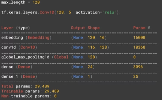
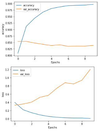
L8 Using a convolutional network

model = tf.keras.Sequential([
    tf.keras.layers.Embedding( vocab_size , embedding_dim , input_length = max_length),
    tf.keras.layers.Conv1D(128, 5 , activation = 'relu'),
    tf.keras.layers.GlobalMaxPooling1D(),
    tf.keras.layers.Dense(24, activation='relu'),
    tf.keras.layers.Dense(1, activation='sigmoid')
    ])

L9 Going back to the IMDB dataset

C3_W3_Lab_4_imdb_reviews_with_GRU_LSTM_Conv1D.ipynb 코드 바로가기

dataset : IMDB Reviews dataset with full word encoding

Embedding layer 후에 Flatten , LSTM , GRU 그리고 Conv1D 같은 다양한 레이어를 실험해보면서 성능을 테스트 해보자.

Import library

import tensorflow_datasets as tfds
import tensorflow as tf
import numpy as np

from tensorflow.keras.preprocessing.text import Tokenizer
from tensorflow.keras.preprocessing.sequence import pad_sequences

data 다운로드 및 준비하기

# Download the plain text dataset
imdb , info = tfds.load('imdb_reviews',with_info = True , as_supervised = True )

# Get the train and test sets
train_data , test_data = imdb['train'] , imdb['test']

# Intitialize sentences and labels lists
training_sentences = []
training_labels = []

testing_sentences = []
testing_labels = []

# Loop over all test examples and save the sentences and labels 

for s , l in test_data:
    testing_sentences.append(s.numpy().decode('utf8'))
    testing_labels.append(l.numpy())
    
# Convert labels lists to numpy array
training_labels_final = np.array(training_labels)
testing_labels_final = np.array(testing_labels)

이전 랩에서는 encoding 된 subword 를 사용했었다. 이번에는 Tokenize 와 padding 과정을 직접 해야 한다.

# Parameters
vocab_size = 10000
max_length = 120
trunc_type = 'post'
oov_tok = "<OOV>"

# Initialize the Tokenizer class
tokenizer = Tokenizer(num_words = vocab_size , oov_token = oov_tok ) 

# Generate the word index dictionary for the training sentences 
tokenizer.fit_on_texts(training_sentences)
word_index = tokenizer.word_index

# Generate and pad the training sequences
sequences = tokenizer.texts_to_sequences(training_sequencesx)
padded = pad_sequences( sequences , maxlen = max_length , truncating = trunc_type ) 

# Generate and pad the test sequences
testing_sequences = tokenizer.texts_to_sequences(testing_sentences ) 
testing_padded = pad_sequences ( testing_sequences , maxlen = max_length )

Model1 : Flatten

장점 : 학습속도가 빠르다.

# Parameters
embedding_dim = 16
dense_dim = 6

# Model Definition with a Flatten layer
model_flatten = tf.keras.Sequential([
    tf.keras.layers.Embedding(vocab_size , embedding_dim , input_length = max_length ) ,
    tf.keras.layers.Flatten(),
    tf.keras.layers.Dense(dense_dim , activation = 'relu'),
    tf.keras.layers.Dense( 1, activation = 'sigmoid')
    ])
    
    # Set the training parameters
    model_flatten.compile(loss='binary_crossentropy' , optimizer= 'adam', metrics = ['accuracy'])
    
    # Print the model summary
    model_flatten.summary()

NUM_EPOCHS = 10 
BATCH_SIZE = 128

# Train the model
history_flatten = model_flatten.fit(padded , training_labels_final , batch_size = BATCH_SIZE , epochs = NUM_EPOCHS , validation_Data = ( testing_padded, testing_labels_final))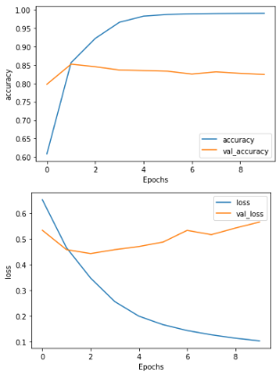

Model2 : LSTM

속도는 느리지만 , 토큰의 순서가 중요한 애플리케이션에서 유용하다.

# Parameters 
embedding_dim = 16
lstm_dim = 32
dense_dim = 6

# Model Definition with LSTM
model_lstm = tf.keras.Sequential([
    tf.keras.layers.Embedding(vocab_size , embedding_dim , input_length = max_length),
    tf.keras.layers.Bidirectional(tf.keras.layer.LSTM(lstm_dim)),
    tf.keras.layers.Dense(dense_dim, activation = 'relu'),
    tf.keras.layers.Dense(1, activation = 'sigmoid')
    ])
    
 # Set the training parameters
 model_lstm.compile(loss = 'binary_crossentropy', optimizer = 'adam', metrics=['accuracy'])
 
 # Print the model summary
 model_lstm.summary()

Model 3 : GRU ( Gated Recurrent Unit )

단순한 LSTM 버전
시퀀스가 중요한 애플리케이션에서 사용할 수 있다.
정확도가 떨어지는 대신 속도가 빠르다.
- model summary 를 보면 LSTM 보다 작고 몇 초 더 빠른 학습시간을 볼 수 있다.

import tensorflow as tf

# Parameters
embedding_dim = 16
gru_dim = 32
dense_dim = 6

# Model Definition with GRU
model_gru = tf.keras.Sequential([
    tf.keras.layers.Embedding(vocab_size, embedding_dim, input_length=max_length),
    tf.keras.layers.Bidirectional(tf.keras.layers.GRU(gru_dim)),
    tf.keras.layers.Dense(dense_dim, activation='relu'),
    tf.keras.layers.Dense(1, activation='sigmoid')
])

# Set the training parameters
model_gru.compile(loss='binary_crossentropy',optimizer='adam',metrics=['accuracy'])

# Print the model summary
model_gru.summary()

Model 4 : Convolution

데이터셋으로부터 특징을 추출하기 위한 convolution layer
GlobalAveragePooling1d layer 를 추가하여 dense layer 전에 결과 값을 줄일 수 있다.
Flatten 을 사용한 모델과 같이 LSTM,GRU 같은 RNN layer 를 사용한 다른 모델 보다 빠르다.

# Parameters
embedding_dim = 16
filters = 128
kernel_size = 5
dense_dim = 6

# Model Definition with Conv1D
model_conv = tf.keras.Sequential([
    tf.keras.layers.Embedding(vocab_size, embedding_dim, input_length=max_length),
    tf.keras.layers.Conv1D(filters, kernel_size, activation='relu'),
    tf.keras.layers.GlobalAveragePooling1D(),
    tf.keras.layers.Dense(dense_dim, activation='relu'),
    tf.keras.layers.Dense(1, activation='sigmoid')
])

# Set the training parameters
model_conv.compile(loss='binary_crossentropy',optimizer='adam',metrics=['accuracy'])

# Print the model summary
model_conv.summary()

L10 Tips from Laurence

text dataset 은 image dataset 보다 overfitting에 빠지기 쉽다.

text dataset 의 validation set에는 training set 에 없는 단어들이 많이 등장할 수 있기 때문
overfitting 을 방지할 수 있는 방법에는 어떤 것들이 있는지 알아보자

C3_W3_Lab_5_sarcasm_with_bi_LSTM.ipynb 코드 바로가기

dataset: News Headlines Dataset for Sarcasm Detection

Bi-LSTM Model 을 학습시켜보자.

Data Preprocessing

import numpy as np
from tensorflow.keras.preprocessing.text import Tokenizer
from tensorflow.keras.preprocessing.sequence import pad_sequences

vocab_size = 10000
max_length = 120
trunc_type = 'post'
padding_type = 'post'
oov_tok = "<OOV>"

# Initialize the Tokenizer class 
tokenizer = Tokenizer(num_words = vocab_size , oov_token = oov_tok

# Generate the word index dictioonary
tokenizer.fit_on_texts(training_sentences)
word_index = tokenizer.word_index

# Generate and pad the training sequences
training_sequences = tokenizer.texts_to_sequences( training_sentences)
training_padded = pad_sequences(training_sequences , maxlen = max_length , padding = padding_type , truncating=trunc_type)

# Generate and pad the testing sequences
testing_sequences = tokenizer.texts_to_sequences(testing_sentences)
testing_padded = pad_sequences(testing_sequences , maxlen=max_length , padding = padding_type , truncating = trunc_type)

# Convert the labels lists into numpy arrays
training_labels = np.array(training_labels)
testing_labels = np.array(testing_labels)

Build and Compile the Model

아래 모델은 IMDB Reviews dataset 을 다룰 때 썼던 것과 거의 유사하다. parameters 를 바꾸면서 training time 과 accuracy 에 어떤 영향이 있는지 살펴보자.

import tensorflow as tf

# Parameters
embedding_dim = 16
lstm_dim = 32
dense_dim = 24

# Model Definition with LSTM
model_lstm = tf.keras.Sequential( [
    tf.keras.layers.Embedding(vocab_size, embedding_dim , input_length = max_length),
    tf.keras.layers.Bidirectional(tf.keras.layers.LSTM(lstm_dim)),
    tf.keras.layers.Dense(dense_dim,activaiton='relu'),
    tf.keras.layers.Dense(1,activation='sigmoid')
    ])
    
# Set the training parameters
model_lstm.compile(loss='binary_crossentropy', optimizer='adam', metrics=['accuracy'])

# Print the model summary
model_lstm.summary()

Training the model

NUM_EPOCHS = 10

# Train the model 
history_lstm = model_lstm.fit(training_padded, training_labels , epochs = NUM_EPOCHS , validation_data = (testing_padded , testing_labels))

Test

dense_dim = 6
- 과적합 양상이 뚜렷해짐

dense_dim = 256
- 훈련속도가 느려짐
- 비슷한 정도의 과적합
lstm_dim = 64
dense_dim = 128
- 처음과 비슷한 훈련속도
- 비슷한 정도의 과적합

C3_W3_Lab_6_sarcasm_with_1D_convolutional.ipynb 코드 바로가기

Lab_5 보다 그래프가 부드러워졌지만 여전히 과적합 양상을 보인다.

Build and Compile the Model

import tensorflow as tf

# Parameters
embedding_dim = 16
filters = 128
kernel_size = 5
dense_dim = 6

# Model Definition with Conv1D
model_conv = tf.keras.Sequential([
    tf.keras.layers.Embedding(vocab_size, embedding_dim, input_length=max_length),
    tf.keras.layers.Conv1D(filters, kernel_size, activation='relu'),
    tf.keras.layers.GlobalMaxPooling1D(),
    tf.keras.layers.Dense(dense_dim, activation='relu'),
    tf.keras.layers.Dense(1, activation='sigmoid')
])

# Set the training parameters
model_conv.compile(loss='binary_crossentropy',optimizer='adam',metrics=['accuracy'])

# Print the model summary
model_conv.summary()

Train the Model

NUM_EPOCHS = 10

# Train the model
history_conv = model_conv.fit(training_padded, training_labels, epochs=NUM_EPOCHS, validation_data=(testing_padded, testing_labels))

Test

kernel_size = 3
dense_dim = 24
- 느려진 학습속도
- overfitting

Quiz

How does an LSTM help understand meaning when words that qualify each other aren’t necessarily beside each other in a sentence?

Values from earlier words can be carried to later ones via a cell state
What’s the best way to avoid overfitting in NLP datasets?

None of the above ( not in LSTMs , GRUs , Conv1D )

Week 3: Exploring Overfitting in NLP

dataset : Sentiment140 dataset

이전 lab 에서와 비슷한 helper function , pre-processing data , tokenize sentences 과정을 거치지만 overfitting 을 방지해보자.

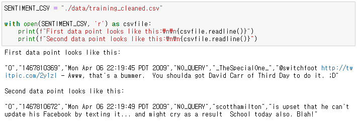
Explore the dataset

각 값은 comma 로 구분되어 있다.

target : 트윗의 긍/부정 ( 0 = negative , 4 = positive )

ids : 트윗의 아이디

date : 트윗 날짜

flag : query , query 가 아니면 NO_QUERY 라는 값을 가진다.

user : 트윗한 유저

text : 트윗 텍스트

Parsing the raw data : `parse_data_from_file` function

조건

헤더가 없으므로 첫 행 생략 x

numpy array 말고 그냥 list 로 저장해도 됨

csv.reader 를 이용해서 파일을 읽기 위해 적절한 arguments 전달

csv.reader 는 각 행을 포함하는 iteration 을반환한다. raw[0] 부터 raw[5] 까지로 각 데이터에 접근 가능하다.

labels 은 string 으로 제공된다. integer 로 변환해서 사용해야함

def parse_data_from_file(filename):
    """
    Extracts sentences and labels from a CSV file
    
    Args:
        filename (string): path to the CSV file
    
    Returns:
        sentences, labels (list of string, list of string): tuple containing lists of sentences and labels
    """
    
    sentences = []
    labels = []
    
    with open(filename , 'r') as csvfile : 
        ### START CODE HERE
        reader = csv.reader(csvfile, delimiter=",")
        
        #for item in reader : 
        #    sentences.append( item[5])
        #    labels.append( int(item[0] ))
        item_list = list(reader)
        
        sentences = [ item[5] for item in item_list ]
        labels = [ 0 if item[0] is '0' else 1 for item in item_list ]
        
        ### END CODE HERE
        
    return sentences, labels

데이터 셋이 아주 크기 때문에 10% 의 데이터만 샘플링하여 사용하자

# Bundle the two lists into a single one
sentences_and_labes = list(zip(sentences , labels ) )

# Perform random sampling
random.seed(42)
sentence_and_labels = random.sample(sentences_and_labels, MAX_EXAMPLES)

# Unpack back into separate lists
sentences , labels = zip(*sentences_and_labels)

print(f'There are {len(sentences)} sentences and {len(labels)} labels after random sampling\n')

Training - Validation Split : `train_val_split`

training 과 validation 으로 데이터 나누기

def train_val_split(sentences , labels , training_split): 
    """
    Splits the dataset into training and validation sets
    
    Args:
        sentences (list of string): lower-cased sentences without stopwords
        labels (list of string): list of labels
        training split (float): proportion of the dataset to convert to include in the train set
    
    Returns:
        train_sentences, validation_sentences, train_labels, validation_labels - lists containing the data splits
    """    
    ### START CODE HERE
    
    # Compute the number of sentences that will be used for training (should be an integer)
    train_size = int(len(sentences) * training_split)

    # Split the sentences and labels into train/validation splits
    train_sentences = sentences[:train_size]
    train_labels = labels[:train_size]

    validation_sentences = sentences[train_size:]
    validation_labels = labels[train_size:]
    
    ### END CODE HERE
    
    return train_sentences, validation_sentences, train_labels, validation_labels

Tokenization - Sequences, truncating and padding : `fit_tokenizer`

training sentences 에 맞추어진 Tokenizer 를 return 하는 함수 구현

def fit_tokenizer(train_sentences , oov_token):
    """
    Instantiates the Tokenizer class on the training sentences
    
    Args:
        train_sentences (list of string): lower-cased sentences without stopwords to be used for training
        oov_token (string) - symbol for the out-of-vocabulary token
    
    Returns:
        tokenizer (object): an instance of the Tokenizer class containing the word-index dictionary
    """
    ### START CODE HERE
    
    # Instantiate the Tokenizer class, passing in the correct value for oov_token
    tokenizer = Tokenizer( oov_token = OOV_TOKEN)
    
    # Fit the tokenizer to the training sentences
    tokenizer.fit_on_texts(train_sentences)
    
    ### END CODE HERE
    
    return tokenizer

def seq_pad_and_trunc(sentences, tokenizer, padding, truncating, maxlen):
    """
    Generates an array of token sequences and pads them to the same length
    
    Args:
        sentences (list of string): list of sentences to tokenize and pad
        tokenizer (object): Tokenizer instance containing the word-index dictionary
        padding (string): type of padding to use
        truncating (string): type of truncating to use
        maxlen (int): maximum length of the token sequence
    
    Returns:
        pad_trunc_sequences (array of int): tokenized sentences padded to the same length
    """        
    ### START CODE HERE
       
    # Convert sentences to sequences
    sequences = tokenizer.texts_to_sequences(sentences)
    
    # Pad the sequences using the correct padding, truncating and maxlen
    pad_trunc_sequences = pad_sequences(sequences , padding = padding , truncating = truncating , maxlen = maxlen)
    
    ### END CODE HERE
    
    return pad_trunc_sequences

pad_sequences 함수는 numpy array 를 반환한다는 걸 기억하자. 그래서 training 과 validation sequences 는 이미 numpy array 로 구성되어 있다.

하지만 label 데이터는 여전히 python list 이다. 모델 학습 전에 numpy array 로 변환하는 과정이 필요하다.

Using pre-defined Embeddings

pre-trained word vectors 를 사용해보자.
스탠포드가 제공한 GloVe의 100 dimension version 을 사용할 것이다.

Define a model that does not overfit

pre-trained embeddings 를 사용할 때 Embedding layer 가 어떻게 구성되는지 확인해보기
아래 layer 들의 조합
마지막 2개의 layer 는 Dense layer
문제를 푸는 데에는 여러가지 방법이 있으므로 , overfit 되지 않는 여러 architecture 들 시도해보기
긴 훈련시간을 피하기 위해 더 단순한 모델 시도해보기. 문제를 해결하기 위한 architecture 는 Dense layer 를 제외하고 보통 3 ~ 4 개의 layer 로 구성되어 있다.

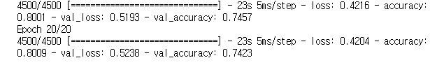
과제를 통과하기 위해서는 val_loss가 평평해지거나 감소해야한다.

아래 이미지와 같이 val_loss 가 평평해지는 것과 train_loss가 낮아지는 것 역시 오버피팅의 지표일 수 있다.

여기서는 아래 이미지와 같이 train_loss는 낮아지는데 val_loss는 높아지는 상황을 방지하고자 한다.

    model = tf.keras.Sequential([ 
        # This is how you need to set the Embedding layer when using pre-trained embeddings
        tf.keras.layers.Embedding(vocab_size+1, embedding_dim, input_length=maxlen, weights=[embeddings_matrix], trainable=False), 
        tf.keras.layers.Dropout(0.2),
        tf.keras.layers.Conv1D(64, 5, activation='relu'),
        tf.keras.layers.MaxPooling1D(pool_size=4),
        tf.keras.layers.LSTM(64),
        tf.keras.layers.Dense(1, activation='sigmoid')
    ])
    
    model.compile(loss='binary_crossentropy',
                  optimizer='adam',
                  metrics=['accuracy'])

Model Test

( 1 ) 전형적인 overfitting 양상을 보인다.

  model = tf.keras.Sequential([ 
        # This is how you need to set the Embedding layer when using pre-trained embeddings
        tf.keras.layers.Embedding(vocab_size+1, embedding_dim, input_length=maxlen, weights=[embeddings_matrix], trainable=False), 
        tf.keras.layers.Conv1D( filters = 64 , kernel_size = 5 , activation='relu'),
        tf.keras.layers.GlobalMaxPooling1D(),
        tf.keras.layers.Dense(128, activation='relu'),
        tf.keras.layers.Dense(1, activation='sigmoid')
    ])

( 2 ) ( 1 ) 모델에 Dropout 추가

    model = tf.keras.Sequential([ 
        # This is how you need to set the Embedding layer when using pre-trained embeddings
        tf.keras.layers.Embedding(vocab_size+1, embedding_dim, input_length=maxlen, weights=[embeddings_matrix], trainable=False), 
        tf.keras.layers.Conv1D( filters = 64 , kernel_size = 5 , activation='relu'),
        tf.keras.layers.GlobalMaxPooling1D(),
        tf.keras.layers.Dropout(0.2),
        tf.keras.layers.Dense(128, activation='relu'),
        tf.keras.layers.Dense(1, activation='sigmoid')
    ])

윰진

이전 포스트

[Coursera] C3W2 Neural Language Processing in TensorFlow - Word Embedding

다음 포스트

[Coursera] C3W3 Neural Language Processing in TensorFlow - Sequence models

DeepLearning.AI TensorFlow Developer

L2 Introduction

L3 LSTMs ( Long Short Turm Memorys )

L4 Implementing LSTMs in code

C3_W3_Lab_1_single_layer_LSTM.ipynb 코드 바로가기

데이터셋 로드하기

데이터셋 준비하기

모델 구성하고 컴파일 하기

모델 훈련시키기

그래프 그리기

C3_W3_Lab_2_multiple_layer_LSTM.ipynb 코드 바로가기

Build and Compile the Model

LSTM architecure 쌓기

Train the Model

시각화

L5 Accuracy and loss

C3_W3_Lab_3_Conv1D.ipynb 코드 바로가기

Build the Model

Train the model

L7 Looking into the code

L8 Using a convolutional network

L9 Going back to the IMDB dataset

C3_W3_Lab_4_imdb_reviews_with_GRU_LSTM_Conv1D.ipynb 코드 바로가기

Import library

data 다운로드 및 준비하기

Model1 : Flatten

Model2 : LSTM

Model 3 : GRU ( Gated Recurrent Unit )

Model 4 : Convolution

L10 Tips from Laurence

C3_W3_Lab_5_sarcasm_with_bi_LSTM.ipynb 코드 바로가기

Data Preprocessing

Build and Compile the Model

Training the model

Test

C3_W3_Lab_6_sarcasm_with_1D_convolutional.ipynb 코드 바로가기

Build and Compile the Model

Train the Model

Test

Quiz

Week 3: Exploring Overfitting in NLP

Explore the dataset

Parsing the raw data : parse_data_from_file function

Training - Validation Split : train_val_split

Tokenization - Sequences, truncating and padding : fit_tokenizer

Using pre-defined Embeddings

Define a model that does not overfit

Model Test

[Coursera] C3W2 Neural Language Processing in TensorFlow - Word Embedding

[Coursera] C3W4 Neural Language Processing in TensorFlow - Sequence models and literature

0개의 댓글

Parsing the raw data : `parse_data_from_file` function

Training - Validation Split : `train_val_split`

Tokenization - Sequences, truncating and padding : `fit_tokenizer`