[2015 ICML] Batch Normalization : Accelerating Deep Network Training by Reducing Internal Covariate Shift

paper info
Author: Sergey Ioffe, Christian SzegedyConference: ICML 2015(International Conference on Machine Learning)
Abstract
-
Deep Neural Network를 training시키는 것은
training 동안에 각 layer의 input의 distribution이 계속해서 바뀌기 때문에 복잡하다. -
각 layer의 input의 distribution이 계속해서 바뀌는 것은
작은 learning rate와 신중한 parameter initialization이 필요하기 때문에
training을 느리게 만든다. -
우리는 각 layer의 input의 distribution이 계속해서 바뀌는 현상을
internal covariate shift라고 언급한다.
그리고 우리는layer의 input을 normalize함으로써internal covariate shift문제를 다뤘다. -
우리의 방법은 normalization을 model architecture의 일부분으로 만들고,
각 training mini-batch마다 normlization을 수행하는 것이었다. -
Batch Normalization은 더 큰 learning rate와 initialization에 대한 적은 주의를 허용한다.
그리고 또한 regularizer로써의 역할도 한다.
어떤 경우에는 dropout을 제거해도 되는 경우가 있다.
1. Introduction
-
Deep learning은 vision, speech, 또 다른 여러 분야에서 급속도로 발전하고 있다.
Stochastic Gradient Descent(SGD)는 deep network를 training 시키는 효과적인 방법이라고 증명되어져 왔다.
또한 SGD with momentum and Adagrad은
state of the art performance를 달성하는 데에 사용되고 있다. -
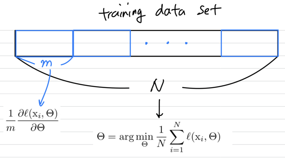
SGD는 training의 각 단계마다 개의 size를 갖는 mini-batch 를 고려하여
-
SGD는 전체 N개()의 training data set에 대하여 loss를 minimization하는 parameter 를 optimize한다.
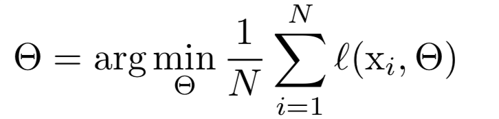 training하는 각각의 단계에서,
개()의 mini-batch는 parameter 에 대한 function의 gradient를 approximation하는 데에 사용된다.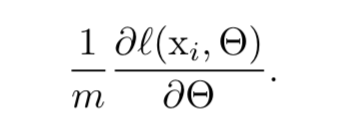
-
한 번에 하나의 example보다, mini-batch를 사용하는 것은 여러가지로 유용하다.
- mini-batch size가 클수록,
mini-batch의 loss에 대한 gradient는 전체 training set에 대한 gradient로 추정할 수 있다. - 현대 computing platform에 있는 parallelism 덕분에 size mini-batch에 대한 computation이
1개의 example을 번 computation하는 것보다 더욱 효율적이다.
- mini-batch size가 클수록,
-
SGD가 simple and effective하긴 하지만,
hyper-parameter tuning하는 데에 주의가 필요하다.
특히 learning rate 뿐만 아니라 parameter의 initial value에 신중해야 한다.
각각의 layer들의 input은 앞선 layer들의 parameter에 영향을 받기 때문에 training이 복잡해진다.
parameter의 작은 변화는 network가 깊어질수록 증폭된다. -
layer input의 distribution에 대한 변화는 문제가 된다.
왜냐하면 layer들은 계속해서 new distribution에 적응해야 하기 때문이다.
learning system에 대한 input distribution이 변화할 때, 이를covariate shift라고 부른다.
(Improving predictive inference under covariate shift by weighting the log-likelihood function) -
covariate shift 개념은 전체의 learning system을 넘어,
sub-network 또는 하나의 layer로 확장되어질 수 있다.
network computing을 고려해보자.
는 임의의 transformation이고,
parameter 는 를 minimization하기 위해 학습되어진다.
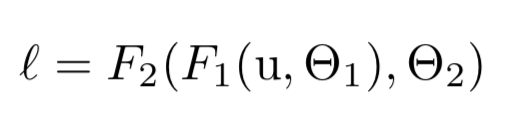 를 라 했을때,
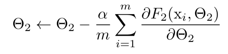
를 learning하는 것은 를 sub-network에 입력하는 것으로 볼 수 있다.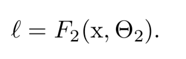 예를 들어, gradient descent 단계(batch size : , learning rate : )는
단독의 network 에 input 가 들어가는 것과 정확히 똑같다고 볼 수 있다.
 따라서 의 distribution이 시간이 지나도 고정된 상태로 유지되는 것이 유리할 것이다.
그러면 는 의 distributino이 바뀌는 것을 보상하기 위해 재조정할 필요가 없다.
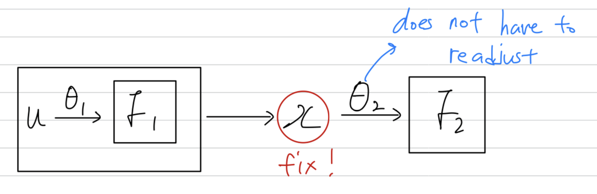
-
또한 sub-network의 input의 distribution을 fix시키면,
그 sub-network의 외부 layer들에게 좋은 결과를 준다.
라는 sigmoid activation function을 가정해보자.
( : layer input, : weight matrix, : bias vector)
는 sigmoid이기 때문에 .
가 증가할수록, 되는 경향이 있다.
이것은 절대값이 작은 dimension을 제외한 모든 의 dimension에 대해서
gradient가 vanishing될 것이고 training 속도가 느려질 것이다.
는 과 layer에 있는 모든 parameter에 의해 영향을 받기 때문에
training 중에 이러한 parameter들의 변경은 의 많은 차원을 saturated regime으로 이동시키고,
convergence를 늦추기 쉽다.
이러한 효과는 network depth가 증가할수록 잘 증폭된다.
실제로 saturation problem과 gradient vanishing 문제는
ReLU 사용, careful initialization(https://proceedings.mlr.press/v9/glorot10a/glorot10a.pdf),
small learning rate 사용으로 어느정도 해결할 수 있지만
network가 훈련하는 동안 nonlinearity input의 distribution이 안정적으로 유지된다면,
optimizer는 saturated regime에 빠질 가능성이 적고, training이 가속화될 수 있을 것이다.
-
우리는 training 동안 deep network의 internel node들의 distribution이 바뀌는 것을
Internal Covariate Shift라고 부른다.
우리는 internal covariate shift를 줄이기 위한 방법으로Batch Normalization이라는 새로운 mechanism을 제안한다.
BN은 layer input의 mean과 variance를 고정시키는 normalization step을 통해 이루어진다. -
BN은 deep neural net의 training을 급격하게 가속화시킨다.
그리고 또한 parameter의 scale과 initial value의 의존성을 줄임으로써 gradient flow에 좋은 영향을 준다.
이는 divergence의 위험 없이 더 큰 learning rate를 사용할 수 있도록 도와준다.
게다가 BN은 model을 regularize하고, dropout의 필요성을 줄여준다.
2. Towards Reducing Internal Covariate Shift
-
training 과정에서 layer들의 input의 distribution을 fixing함으로써,
우리는 training speed 향상을 기대할 수 있다. -
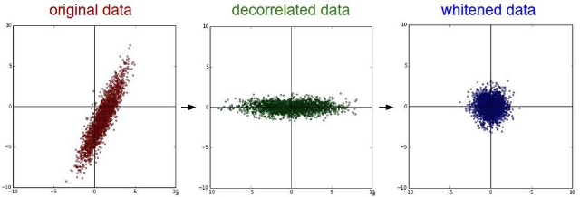
input을 whitened(linearly transformed to have zero means and unit variances)하는 것이 training을 빠르게 만든다는 것을 잘 알고 있다.
(https://cseweb.ucsd.edu/classes/wi08/cse253/Handouts/lecun-98b.pdf)
각 layer의 input을 whitening시킴으로써,
우리는 internal covariate shift의 안좋은 효과를 제거하는 fixed distribution of inputs을 달성하는 데에 한 걸음 다가간 것이다.
하지만 whitening(mean 0, variance 1)을 하는 것은 optimization step에 영향을 줄 수 있다.
gradient descent step은 normalization을 update해야 하는 방식으로 parameter를 update하려고 할 수 있고,
이는 gradient step의 효과를 줄인다.
예를 들어,
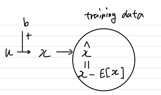
input 에 학습된 bias 를 더하는 layer를 고려해보자.()
그리고 그 layer는 output = 을 training data에 대한 mean을 subtracting하여 normalization한다.
where , {} is the set of values of over the training set, and .
(아래와 같은 layer를 고려)
 만약 gradient descent step이 에 대한 의 의존도를 무시한다면, 다음과 같이 update될 것이다.
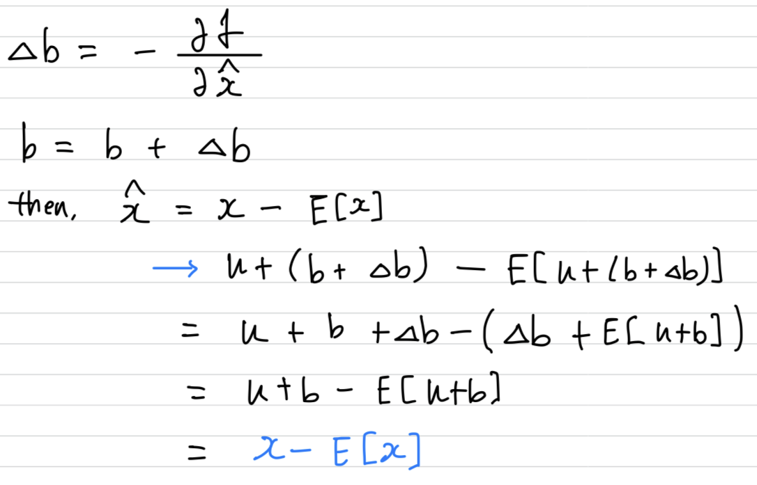 따라서 b의 update와 그에 따른 normalization의 변화는
결과적으로 layer의 output 또는 loss의 아무런 변화도 초래하지 않았다.
➡️ 즉, 일부 parameter의 영향이 무시된다.
traning이 계속된다면, loss가 고정된 채로 계속 는 무한대로 커지게 된다.
우리는 초기 실험에서 이것을 경험적으로 관찰했으며,
normalization parameter가 gradient descent step 밖에서 계산될 때, model은 폭발하게 된다.
Motivation
이렇게 매 layer마다 whitening을 적용하는 것은 비용이 많이 든다.
(computing covariance matrix, iverse squre root, ...)
This motivates us to seek an alternative that performs input normalization in a way
that is differentiable and does not require the analysis of the entire training set
after every parameter update.
3. Normalization via Mini-Batch Statistics
-
각 layer의 input에 모두 whitening을 적용하는 것은 비용이 매우 많이 들고, 어디에서나 미분이 가능하지 않기 때문에
우리는two necessary simplification을 만들었다.-
The first is that instead of whitening the features in layer inputs and jointly,
we will normalize each scalar feature independently, by making it have the mean of zero and the variance of 1.
For a layer with d-dimensional input ,
we will normalize each dimension
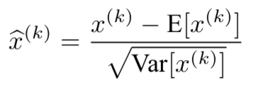 where the expectation and variance are computed over the training data set.
단순히 layer의 각 input을 normalizing하는 것은 그 layer가 represent할 수 있는 것을 바꿀 수 있다.
예를 들어, sigmoid의 input을 normalizing하는 것은 linear regime으로 제한된다.
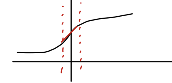 이를 해결하기 위해
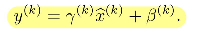
normalizing된 값을 scale, shift 해주기 위한 parameter인 를 만들었다.
-
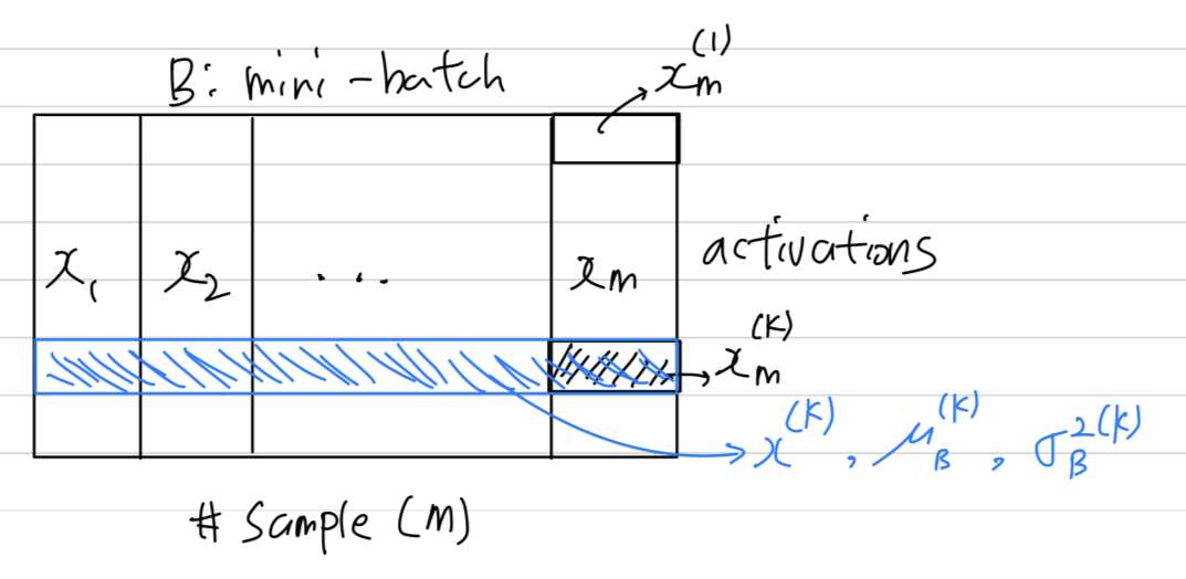
우리는 SGD training에 사용할 mini-batch를 고려한다.
 mini-batch of size .
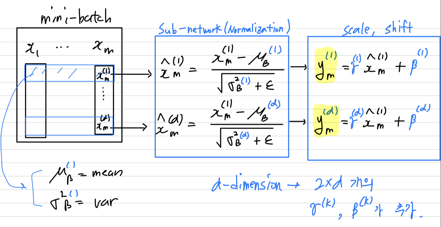
특정 activation인 에 focus하겠다. 그리고 clarity를 위해 로만 표시하겠다.
-
-
-dimension이 있다면, 개 만큼의 learnable parameter인 가 생기는 것임.
또한 BN은 각 training example에 대한 activation을 독립적으로 구하는 것이 아니라,
은 mini-batch 내의 다른 example들에 의존한다. -
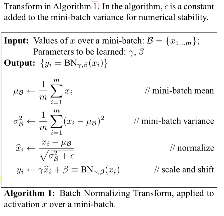
만약 우리가 을 무시한다면,
each normalized activation 는 평균 0, 분산 1을 갖을 거라 예상할 수 있다.
(, )
normalized된 은 sub-network의 training을 빠르게 만들 수 있고, 결국 전체 network의 training을 빠르게 만들 수 있다. -
training하는 동안에,
BN transform으로 인한 loss 의 gradient를 backpropagate해야 하고,
우리는 chain rule을 사용한다.- 논문에서 사용했다고 한 backprop 식 :
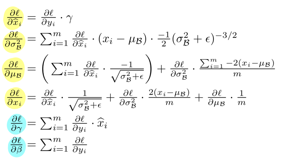
- 내가 해본 backprop 식 :
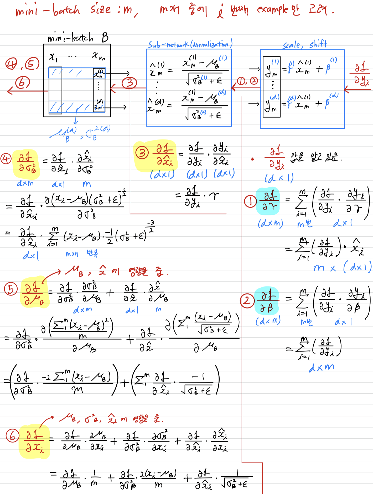 (data flow graph 참고한 곳 : https://www.youtube.com/watch?v=58fuWVu5DVU&t=1304s)
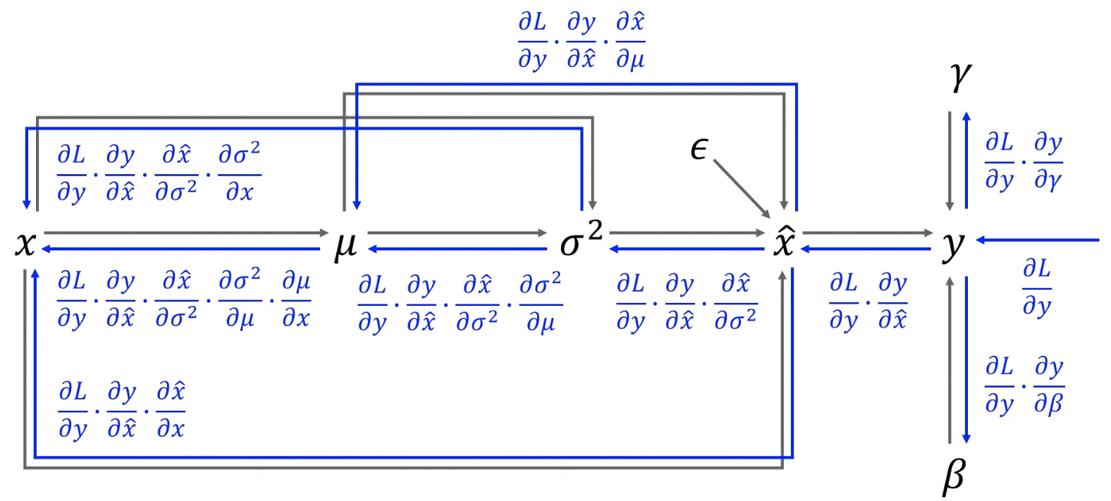
- 논문에서 사용했다고 한 backprop 식 :
3.1 Training and Inference with Batch Normalized Networks
-
우리는 Batch-Nomarlize network를 위해서,
Algorithm 1대로 activations의 subset으로 BN transform을 insert하였다.
이제 라는 input을 받는 layer는 모두 을 input으로 받게 된다. -
BN을 사용하는 model은 batch gradient 또는 mini-batch size가 인 SGD를 사용하여
tain되어질 수 있다. -
mini-batch에 의존하는 activation의 normalization은 효율적인 training이 될 수 있지만,
하지만 inference(test)하는 동안에는 바람직하지 않다.
test 단계에서는 입력 단위가 mini-batch가 아니기 때문에
통계학적인 접근으로 training 단계에서 사용했던 모집단을 이용한 normalization을 사용한다.
그래서 우리는 inference 동안에
unbiased variance estimate: 를 사용한다.
unbiased variance estimate의 기대값은 training하는 동안의 개의 mini-batch에 대한 sample variance(표본 분산)이다.
통계학에서는 여러 이유로 sample variance(표본분산)가 population variance(모분산)을 잘 estimate하도록 하기 위해 variance에 을 곱해준다.
이를 unbiased variance estimate라고 한다. (https://blog.naver.com/sw4r/221021838997)
그리고 training 동안 moving average를 사용하여
inference(test)하는 동안 mean과 variance를 fix시켰다.
또한 scaling하는 와 shift하는 와 함께 linear transform인 을 구성한다. -
다음은 batch-normalized network를 training하기 위한 과정을 요약해 놓은 Algorithm 2이다.
- Algorithm 2의 이해를 더 쉽게 하기 위한 그림
Algorithm 2

- Algorithm 2의 이해를 더 쉽게 하기 위한 그림
3.2 Batch-Normalized Convolutional Networks
-
BN은 network의 어떠한 activation set에나 적용될 수 있다.
예를 들어 다음의 nonlinear activation이 붙어있는 affine transform을 고려해보자.
(where and are learned parameterrs of the model, g() is the nonlinearity such as sigmoid or ReLU)
이 formulation은 FC layer와 convolutional layer 모두 cover할 수 있다.
우리는 nonlineartity 바로 직전에 BN transform을 추가한다.
또한 bias 는 mean을 구하는 과정에서 효과가 없어지기 때문에 없앤다.
따라서 로 바꿀 수 있다. -
convolutional layer의 경우,
mini-batch 은 feature map에 있는 모든 value가 된다.
따라서 mini batch size가 이고, feature map size가 x 라면
우리는 의 유효한 mini-batch를 사용한다.
우리는 각 activation이 아닌, feature map에 대한 와 를 학습한다.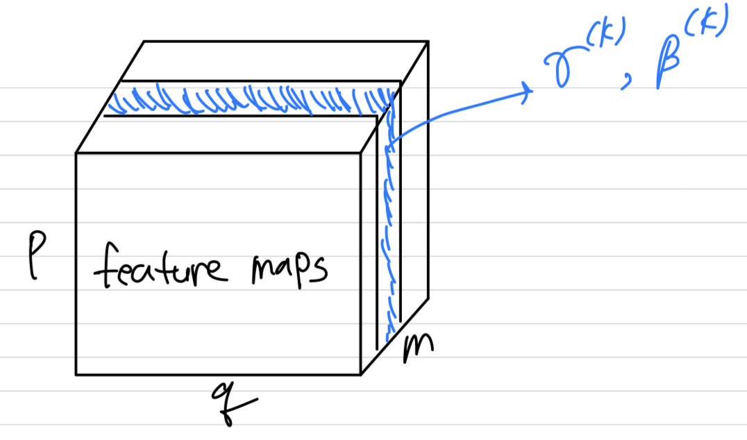
3.3 Batch Normalization enables higher learning rates
-
In traditional deep networks, too-high learning rate may result in the gradients that explode or vanish.
BN helps adress these issues. -
BN은
parameter의 작은 변화가 gradient의 activations에서 더 크고 최적이 아닌 변화로 증폭하는 것을 방지한다.
예를 들어, nonlinearities의 saturated regime에 갇히는 것을 막을 수 있다. -
또한 BN은 parameter scale에 대해 회복력이 있다.
일반적으로 large learning rate는 parameter의 scale을 증가시키고,
커진 parameter값은 backpropagation 과정에서 gradient를 증폭시켜 explosion을 이끈다.
하지만 BN에서는 backpropagation이 parameter의 scale에 영향을 받지 않는다.
3.4 Batch Normalization regularizes the model
- When training with Batch Normalization,
어떠한 training example은 다른 mini-batch에 묶여서 등장하기 때문에,
더 이상 training example에 대해 deterministic(예측한 그대로 동작) 하지 않다.
➡️ (나의 생각) : 이것은 normalization의 효과라기보다는 mini-batch에 대한 효과인 것 같은데
mini-batch가 regularization 효과가 있을까?
4. Experiments
4.1 Activations over time
-
internal covariate shift 현상과 BN의 능력을 증명하기 위해
MNIST dataset을 predicting하는 것을 고려했다. -
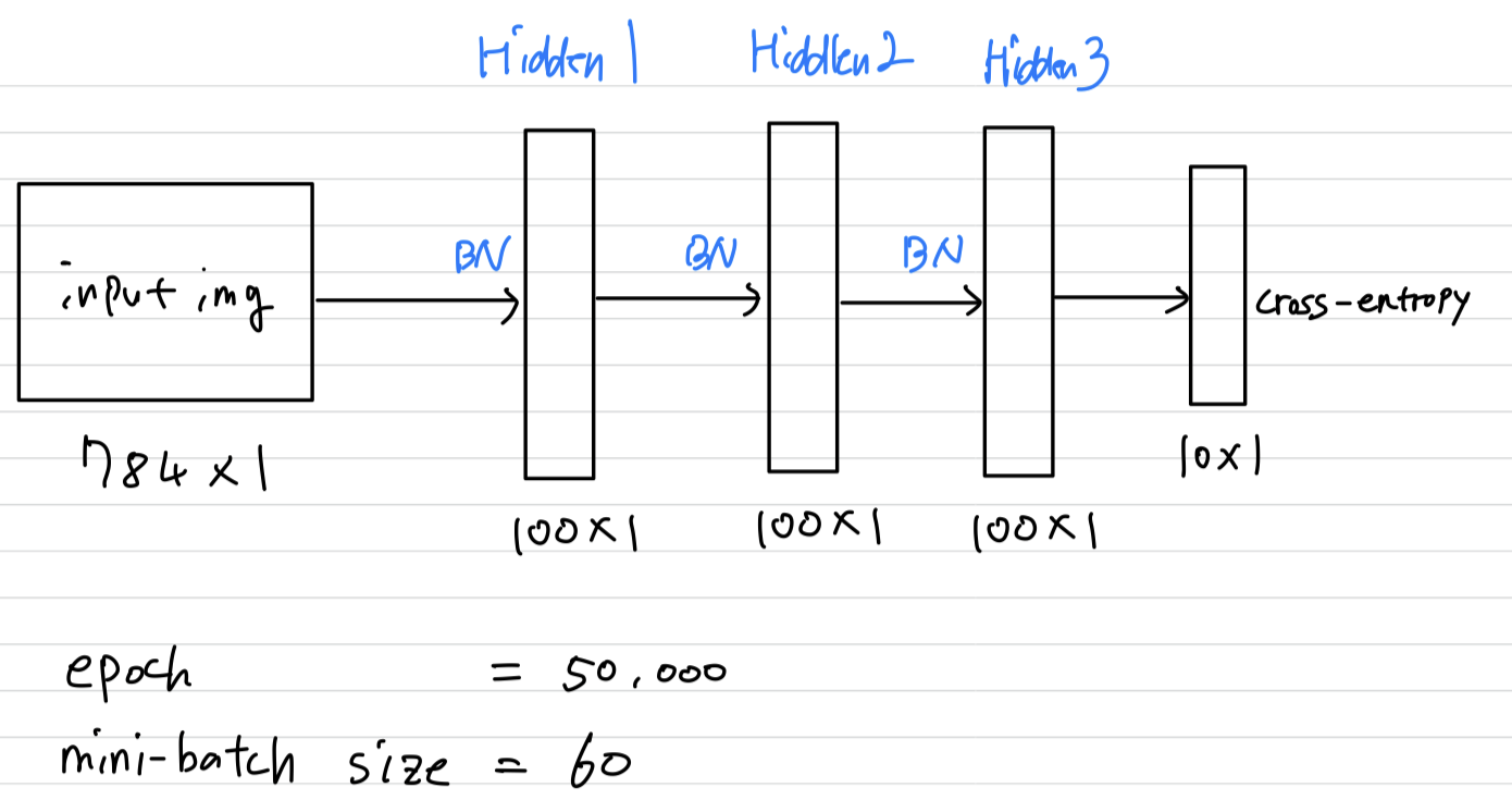
우리는 28 x 28 binary image를 input으로 사용하고,
각각 100개의 activations을 갖는 3개의 FC hidden layer를 사용하는 간단한 network를 만들었다.
각 layer는 를 계산하는 sigmoid nonlinearity를 사용했고,
weights 는 Gaussian 분포를 따르는 작은 random 값으로 initialized했다.
마지막 hidden layer는 10개 activation이 있는 FC layer를 따르고 cross-entropy loss를 사용한다.
우리는 이 network를 50,000 steps으로 train시켰고,
각 mini-batch 당 60개의 examples을 사용했다.
그리고 각 hidden layer에 BN을 적용했다.
 우리는 MNIST에 대한 state of the art performance를 달성하는 것보다,
without BN nework와 with BN network의 비교에 관심이 있었다.
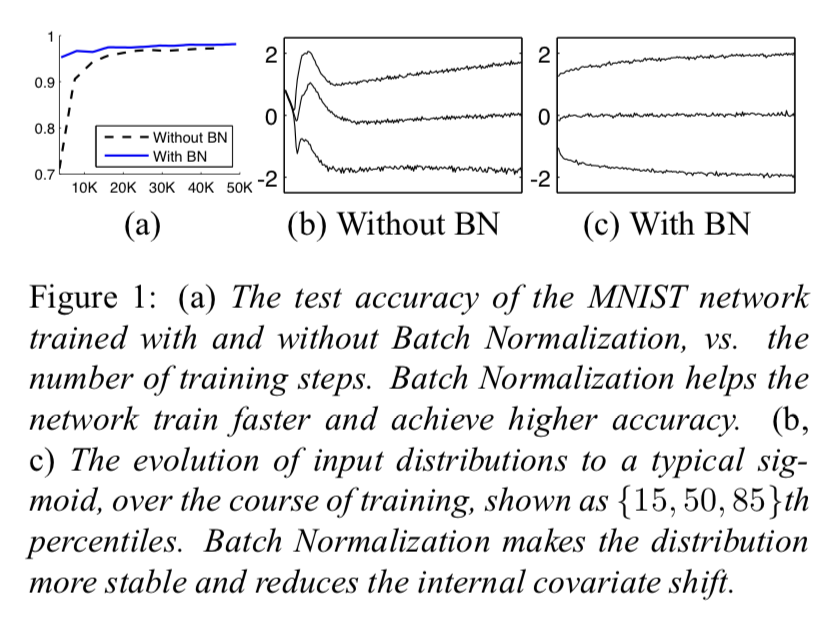
- (a) : MNIST network를 training하는 중에 평가한 test accuracy이다.
Network with BN model이 더욱 빠른 학습과 높은 accuracy를 보인다.
왜 그런지 알아보기 위해 Network without BN과 Network with BN에 대해서,
sigmoid의 input을 관찰해봤다. ➡️ (b), (c) - (b), (c) :
(b), (c)는 각 network의 마지막 hidden layer로부터 특정 activation값 하나를 관찰한 것이다.
그 값의 분포가 어떻게 진화하는지 볼 수 있다.
(b) = Without BN은 mean과 variance가 시간이 지남에 따라 크게 바뀐다.
하지만 (c) = With BN의 distribution은 더욱 안정적이고, 이는 training에 도움을 준다.
- (a) : MNIST network를 training하는 중에 평가한 test accuracy이다.
4.2 ImageNet classification
-
우리는 Inception Network(GoogleNet)에 Batch Normalization을 적용해봤다.
기존 GoogleNet에서 다음을 수정해봤다.
아마 이게 GoogleNet version 2 인듯.- (가장 주요한 수정사항)
5 x 5 convolutional layers are replaced by two consecutive 3 x 3 convolutional layers.
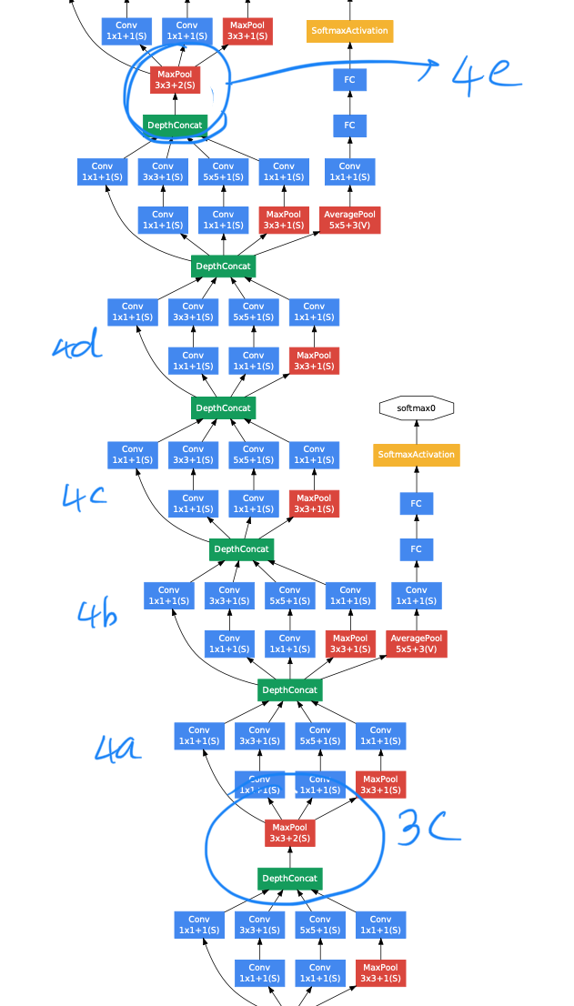
(이는 network의 maximum depth를 증가시킬 수 있었다.) - The number 28 x 28 inception modules is increased 2 to 3.
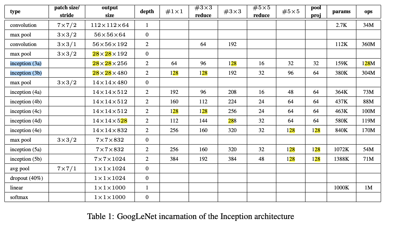 저 drag된 inception module을 2개에서 3개로 늘렸다
➡️ inception (3c)를 추가. - inception module 안에서 어쩔 때는 average pooling, 어쩔 때는 max poolig을 썼다.
- Inception module 사이에 pooling layer를 사용하지 않았지만,
modules (3c), (4e)의 DepthConcat 전에 stride-2 convolution/pooling layer가 사용되었다.
- (가장 주요한 수정사항)
-
On the importance of initial- ization and momentum in deep learning 논문에서 사용했던 momentum과 SGD를 이용하여 학습시켰고,
mini-batch size는 32. -
우리의 실험은
기존 Inception Network에 몇가지 수정을 한 뒤, Batch Normalization을 적용한 것을 평가하는 것이었다. (아마 이게 GoogleNet version 2?)
section 3.2에서 말한 것처럼 convolutional 방법대로, BN을 각 nonlinearity의 input에 적용했다.
4.2.1 Accelerating BN Networks
- 단순히 network에 BN을 적용하는 것만으로는 이 방법의 최대 효율을 끌어내지 못한다.
장점을 극대화하기 위해서는, network와 parameter를 추가적으로 변경해야 한다.Increase learning rate: Sec. 3.3
BN model에서 higher learning rate로부터 더 빠른 학습 속도를 달성할 수 있었다.Remove Dropout: Sec. 3.4
BN은 dropout과 같은 목적을 달성할 수 있다.Reduce the L2 weight regularization:
수정된 BN-Inception network에서 L2 loss의 weight를 로 줄였더니,
validation data에 대한 더 높은 accuracy를 보였다.Accelerate the learning rate decay:
왜나하면 BN-Inception network는 기존 Inception network보다 더 빠르게 학습하기 때문에 learning rate를 6배나 빨리 감소시켰다.Remove Local Response Normalization:
BN을 적용한 network는 Local Response Normalization이 필요하지 않다.
(똑같이 activation에 대해 normalization을 진행하는 것이기 때문에 중복해서 적용하는 꼴이다.
실험상 이는 효과가 없다고 한다.)Shuffle training examples more thoroughly:
우리는 training data에 대해 within-shard shuffling을 가능하게 했다.
이는 하나의 mini-batch에 똑같은 sample example이 나타나는 것을 방지해준다.
이것은 validation accuracy에 대한 1%의 향상을 보였고, BN이 regularizer라는 관점과 일치한다.Reduce the photometric distortions:
batch-normalized network는 학습이 더 빠르기 때문에
network가 "real" image에 더 집중할 수 있도록 image들을 distortion시켰다.
4.2.2 Single-Network Classification
- 우리는 LSVRC2012 training data에 대해 train시킨 다음의 network들을 평가했다.
축 : the number of training steps
축 : the validation accuracy
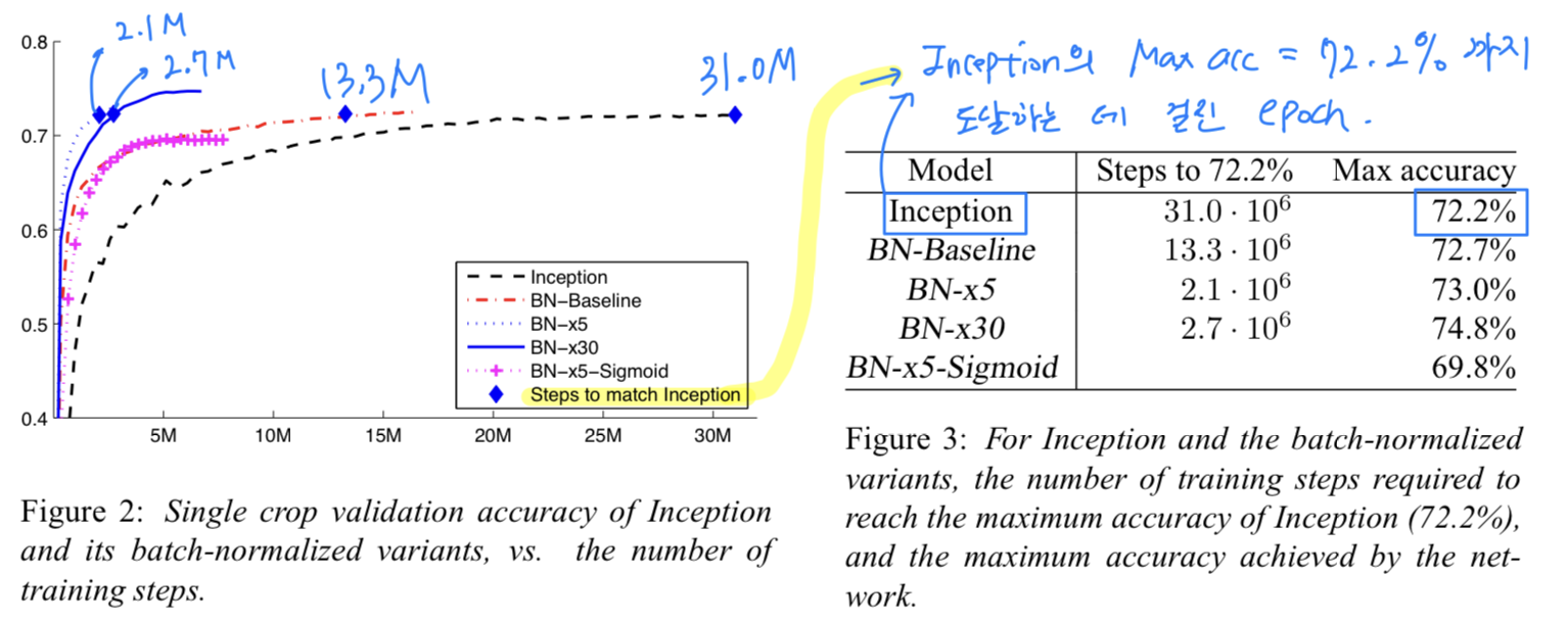
Inception:
BN을 쓰지 않은 기존 Inception network(GoogleNet version 1)
initial learning rate = 0.0015
➡️ 31.3M번 epoch을 돌려야 72.2% accuracy에 도달.
BN-Baseline: Same as Inception with BN before each nonlinearity
➡️ 13.3M번 epoch을 돌려야 72.2% accuracy에 도달.
BN-x5: Inception with BN and the midifications in Sec. 4.2.1.
The initial learning rate was increased by a factor of 5, to 0.0075.
initial learning rate = (5배 증가한 0.0075)
➡️ 2.1M번 epoch을 돌려야 72.2% accuracy에 도달.
BN-x30:
BN-x5과 똑같은데, initial learning rate만 다름
initial learning rate = (30배 증가한 0.045)
➡️ 2.7M번 epoch을 돌려야 72.2% accuracy에 도달.
➡️ (BN-x5보다) learning rate가 더 큰데도 불구하고, 초기에 다소 학습속도가 느림.
하지만 Max accuracy는 더 높음. (74.8 > 73.0)
BN-x5-Sigmoid:
BN-x5과 똑같은데, ReLU 대신 Sigmoid nonlinearity를 사용.
➡️ 72.7% accuracy에 도달하지 못하지만,
BN이 없었다면 Inception with sigmoid는 0.001%의 accuracy도 이루기 힘듦.
4.2.3 Ensemble Classification
-
현재(당시) ILSVRC에서 best result로 보고된 model은
Deep Image ensemble of traditional models과 그 ensemble model이다.
이 ensemble model은 ILSVRC server에서 top-5 error of 4.94%로 평가되었다. -
우리는 ILSVRC server에 따르면
top-5 validation error of 4.9% and test error of 4.82%를 받았다.
(new state-of-the-art)
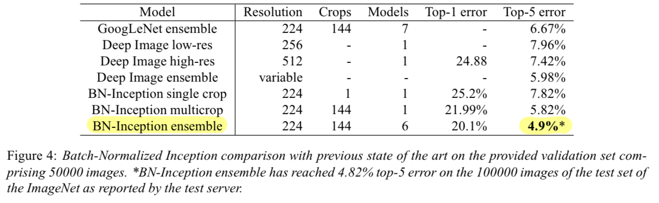
- 우리의 ensemble은 6개의 network를 사용했고, 각각의 model은 조금씩 수정된 BN-x30을 사용했다.
수정된 사항은 다음과 같다.- increased initial weights in the conv layers
- using dropout(probability : 5% or 10%)
- last hidden layer에서는 non-convolutional, per-activation BN.
- 6개 각각의 network는 6M번의 epoch 뒤에 각각의 maximum accuracy를 달성했다.
- ensemble prediction에 대한 detail은 GoogleNet에서와 똑같이 했다.
5. Conclusion
-
우리는 deep network를 학습시키는 데에 급격하게 가속화시킬 수 있는 새로운 mechanism을 발표했다.
-
machine learning system에서 training을 복잡하게 하는 것으로 알려진,
covariate shift가 sub-network와 layer에도 적용되며,
network 내부 activation에서 이를 제거하는 것이 training에 도움이 될 수 있다는 것을 전제로 한다. -
우리가 제안한 method는 activations을 normalizing하고,
이 normalization을 전체 network architecture에 적용함으로써 network의 능력을 끌어낸다. -
deep network training에서 stochastic optimization method가 흔히 사용되게 하기 위해서,
우리는 normalization을 각각의 mini-batch에 적용했고,
normalization parameters를 통해 gradient를 backpropagate했다.
Batch Normalization은 각 activation에 대해 오로지 2개의 추가적인 parameter만 추가하면 된다.
그리고 이렇게 하는 것은 network의 representation ability를 보존한다. -
결과적으로 network는 saturating nonlinearities로 훈련되어질 수 있고,
increased training rate에 더욱 관대하고, 가끔은 dropout이 필요하지 않다. -
이번 연구에서, 우리는 BN에 대한 잠재적으로 가능한 모든 가능성을 살펴보지 않았다.
우리의 향후 연구에는 internal covariate shift와 gradient vanishing or exploding이 특히 심할 수 있는 Recurrent Neural Network에 대한 적용이 포함되며,
이를 통해 BN이 gradient propagatoin를 개선한다는 가설을 보다 철저하게 test할 수 있을 것이다.
이처럼 우리는 알고리즘에 대한 추가 이론적 분석이 더 많은 개선과 적용을 가능하게 할 것이라고 믿는다.
궁금한 점, 모르겠는 부분
-
whitening을 사용할 때의 문제?를 모르겠음.
whitening으로 input의 distribution을 fix시킬 수 있지만,
여러 이유로 문제가 있기 때문에Batch Normalization을 연구한 것임.
(whitening 방법을 개선하고자 한 것이 motivation인 것은 알겠음...) -
coursera에서 BN의 계산방식은 하나의 독립적인 example의 activation 안에서 BN을 수행했었는데,
내가 이해한 이 논문에서의 BN은 다른 example들과의 같은 위치에 pixel값으로 BN을 수행한다.
내가 이 논문에서 이해한게 맞는 것 같은데 coursera에서의 BN과 계산방식이 다르기 때문에 확신이 서지는 않는다..
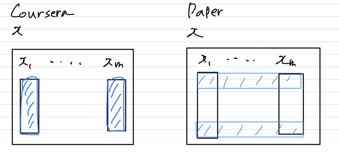
➡️ Coursera에서 잘못된 설명이었거나, 내가 Coursera를 잘못 이해했던 것
➡️ BN paper를 읽으며 이해한 BN 방법이 맞는 방법이다.
