Paper Info

• https://openaccess.thecvf.com/content/CVPR2023/papers/Lin_DynamicDet_A_Unified_Dynamic_Architecture_for_Object_Detection_CVPR_2023_paper.pdf

• Lin, Zhihao, et al. "Dynamicdet: A unified dynamic architecture for object detection." Proceedings of the IEEE/CVF Conference on Computer Vision and Pattern Recognition. 2023.

Abstract

• Dynamic neural network는 DL에서 떠오르는 연구 주제이다.
  adaptive inference를 통해, dynamic models은 놀라운 accuracy and computational efficiency를 달성할 수 있다.
  그러나 object detection을 위한 powerful dynamic detector를 설계하는 것은
  적절한 dynamic architecture와 exiting criterion(종료 기준)이 없기 때문에 challenging하다.

• 이러한 어려움을 해결하기 위해,
  우리는 DynamicDet이라는 a dynamic framework for object detection을 제안한다.

  • 먼저,
    object detection task의 특성에 기반하여 dynamic architecture를 신중하게 설계한다.
  • 그런 다음,
    multi-scale information을 분석하고 inference route(경로)를 자동으로 결정하는 adaptive router를 제안한다.
  • 또한,
    dynamic detectors를 위한 detection losses를 기반으로 한 exiting criterion(종료 기준)을 갖춘 새로운 optimization strategy를 제시한다.
  • 마지막으로,
    하나의 dynamic detector만으로도 넓은 범위의 accuracy-speed trade-off를 실현할 수 있는 variable-speed(가변 속도) inference strategy를 제시한다.

• https://github.com/VDIGPKU/DynamicDet

---

1. Introduction

• object detection은 많은 vision tasks 분야에서 사용되고 있는 필수적인 분야이다.
  최근에, more accurate and faster detectors로 발전되고 있다.
  (예를 들어, Network Architecture Search(NAS)-based detectors and YOLO series models.)
  하지만 이러한 방법들은 accuracy and speed 사이의 좋은 trade-offs를 이루기 위해 여러 model들을 design and train해야 한다.
  이는 다양한 application scenarios에 충분히 flexible하지 않다.
  
  이 문제를 완화하기 위해, 우리는 object detection task를 위한 dynamic inference에 초점을 맞추고,
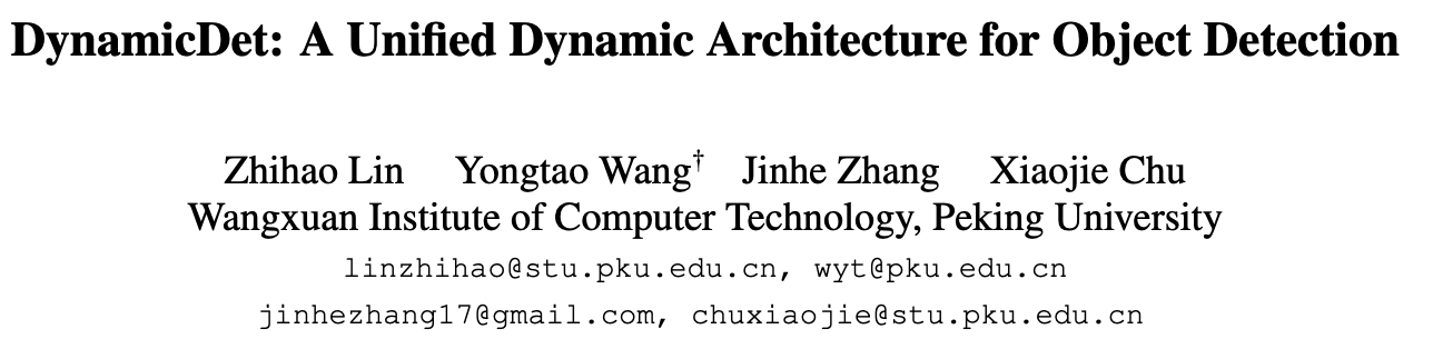
  단 하나의 dynamic detector를 사용하여 넓은 범위의 good accuracy-speed trade-offs를 이루려고 시도했다. (Fig.1)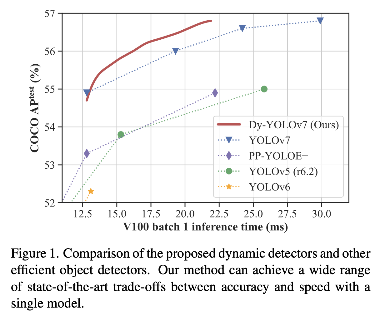

• 인간의 두뇌는 deep learning 분야에서 많은 영감을 주고 있으며, dynamic neural network([12])가 그 대표적인 예시이다.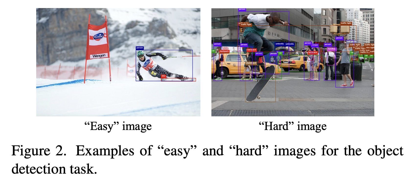Fig. 2의 두 가지 예를 보면,
  우리는 왼쪽의 "easy" image에서는 모든 object를 빠르게 식별할 수 있지만,
  오른쪽 image에서는 같은 효과를 달성하는 데에 더 많은 시간이 필요하다.
  즉, 우리 두뇌에서 image의 처리 속도는 image의 difficulties(난이도)에 따라 다르다.
  이 특성은 image-wise dynamic neural network의 motivation이 되며,
  많은 흥미로운 연구들이 제안되어왔다. (e.g., Branchnet, MSDNet, DVT).
  비록 이러한 접근법들이 놀라운 성능을 달성했지만, 모두 image classification task를 위해 설계되었으며 다른 vision task, 특히 object detection에는 적합하지 않다.

image-wise dynamic detector를 설계하는 주요 어려움은 다음과 같다.

1. Dynamic detectors cannot utilize the existing dynamic architectures.

   • 대부분의 기존 dynamic architecture는 여러 stage(i.e., a stack of multiple layers)로 연결되어 있으며, 각 exiting point에서 inference를 stop할지 여부를 예측한다.
     이러한 paradigm은 image classification에서는 가능하지만 object detection에서는 효과적이지 않다.
     왜냐하면 하나의 image에는 여러 objects가 있고, 각 object에는 보통 다른 category와 scales을 가지고 있기 때문이다.
     따라서 거의 모든 detector들은 여러 sizes의 정보를 활용하여(backbone의 여러 stage에서의 feature를 fusion하여 i.e., FPN),
     object를 detection한다.
     이 경우, detectors의 exiting points는 마지막 stage 뒤에만 위치할 수 있다.
     결과적으로 전체 backbone module을 완전히 실행해야 하며, 여러 stage에 걸친 dynamic inference를 수행하는 것은 불가능하다.

2. Dynamic detectors cannot exploit the existing exiting criteria for image classification.

   • image classification task의 경우,
     Top-1 accuracy의 threshold가 decision-making을 위해 널리 사용되는 기준이다.
     특히, intermediate layer에서 top-1 accuracy를 예측하는 데에 하나의 FC layer만 필요하여 easy and costless하다.
     그러나,
     object detection task는 object instance의 categories and locations을 예측하기 위해 neck과 head가 필요하다.
     따라서 image classification에 사용되는 기존의 exiting criteria는 object detection에 적합하지 않다.

• 위 문제들을 해결하기 위해,
  object detection을 위한 dynamic inference를 실현하는 dynamic framework를 제안한다.
  이를 DynamicDet이라고 한다.
  먼저, inference 중 multi-scale information을 갖고 exit할 수 있는 object detection task를 위한 dynamic architecture를 design했다.
  그 다음, 각 image에 대해 best route를 자동으로 선택하는 adaptive router를 제안한다.
  또한, 제안된 DynamicDet을 위한 optimization and inference strategies도 제시한다.
  우리의 main contribution은 다음과 같다.
  • DynamicDet이라는 dynamic architecture를 제안한다.
    이 architecture는 두 개의 cascaded detectros와 하나의 router로 구성되어 있다.
    이 dynamic architecture는 Faster R-CNN 및 YOLO와 같은 mainstream detectors에 쉽게 적용할 수 있다.
  • image의 difficulty score를 multi-scale feature에 기반하여 예측하고
    automatic decision-making을 할 수 있는 adaptive router를 제안한다.
    또한, dynamic architecture를 위한 hyperparameter가 없는 optimization strategy와 variable-speed inference strategy를 제안한다.
  • 광범위한 실험을 통해 DynamicDet이 단 하나의 dynamic detector로도 다양한 accuracy-speed trade-offs를 얻을 수 있음을 보여준다.
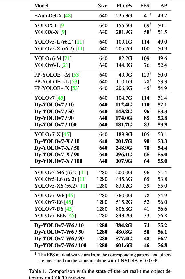
    real-time object detection에서 SOTA를 달성했다. (i.e., 56.8% AP at 46 FPS)

---

2. Related Work

2.1. Backbone design on object detection

• object detector의 성능은 backbone이 추출하는 multi-scale features에 크게 의존하기 때문에
  backbone은 object detection에서 매우 중요한 역할을 한다.
  ResNet과 그 variants(e.g., ResNeXt, Res2Net)은 residual connection을 neural networks에 도입하여
  모든 vision task에 high-quality backbone architecture family를 제공한다.
  더 나아가, calculation load를 줄이기 위해 CSPNet은 duplicate(중복된) gradient information을 줄여
  heavy inference를 감소시키고 efficiency를 크게 증가시켰다.
  이 효과적인 architecture는 많은 lightweight detector(e.g., YOLO series models)에 영감을 주었다.
  이후, global information을 더 잘 학습하기 위해 일부 transformer-based backbones(e.g., PVT, Swin Transformer)들이 제안되었다.
  또한 object detection을 위해 auto-designed backbones들도 제안되었다.
  예를 들어, DetNAS는 object detection task의 guidance에 따라 optimal backbone을 탐색하기 위해 one-shot suprenet을 활용한다.

• 비록 많은 종류의 backbone이 제안되어왔지만,
  거의 모든 backbone이 one set of multi-scale features를 순차적으로 생성하는
  single-pass architecture이기 때문에 모든 stages가 skip될 수 없다.
  다행히도 일부 연구에서는 multiple cascaded backbones architecture를 제안하여 dynamic backbone으로 변환할 가능성을 제시한다.
  예를 들어,
  CBNet은 많은 identical(동일한) backbones을
  composite(복합) connections로 group화하여
  더 강력한 composite backbone을 만든다.
  이러한 backbone은 multiple sub-backbones을 가지고 있으며
  각 sub-backbone은 intermediate multi-scale features를 생성할 수 있으므로,
  dynamic inference를 위해 exiting points를 추가할 수 있다.

2.2. Accuracy-speed trade-off on object detection

• 거의 모든 detection method들은 더 나은 accuracy-speed trade-off를 위해 설계되었다.
  주어진 detector에서, acc-speed trade-off를 얻는 가장 간단한 방법은 model scaling technique들을 채택하는 것이다. (e.g., channel size를 늘리거나 layer를 반복)
  EfficientDet은 모든 module의 resolution, depth, width를 동시에 균일하게 scaling하여
  real-time detector에서 놀라운 efficiency를 달성했다.
  Sclaed-YOLOv4는 더 나은 trade-off를 추구하기 위해 depth, width, resolution 뿐만 아니라 network structure도 수정했다.
  YOLOv7은 concatenation-based model을 위해 compound scaling method를 설계하여 SOTA를 달성했다.
  EAutoDet은 supernet을 구축하고 다양한 HW constraints에서 적절한 scaling factor를
  자동으로 검색하기 위해 Network Architecture Search(NAS)를 채택했다.

• 그러나 위의 모든 방법은 best trade-offs를 위해 여러 detector들을 훈련해야 한다.
  (e.g., real-time detection을 위한 하나의 tiny model과 정확한 detection을 위한 또 다른 large model)
  이는 막대한 training resource를 필요로 한다.
  본 논문에서는 dynamic detector에 중점을 두고 하나의 dynamic detector로 광범위한 accuracy-speed trade-offs를 달성하는 것을 목표로 한다.

2.3. Dynamic neural network

• dynamic neural network는 image별 또는 pixels별로 adaptive computation을 할 수 있다.

  • SACT는 일반적인 spatial-wise dynamic network이고, image의 특정 region에 따라 실행한 layer의 수를 적절히 조절하여 network의 efficiency를 개선했다.
    그러나 SACT의 실제 speed-up 성능은 hardware-software co-design에 크게 의존한다.
    현재의 DL HW와 libraries는 이러한 spatial -wise dynamic networks를 잘 지원하지 않는다.
  • 반면, image-wise dynamic network는 sparse computing에 의존하지 않으며,
    기존의 CPU와 GPU에서 쉽게 accelerated될 수 있다.
    예를 들어, Branchynet은 model이 intermediate layer에서 충분히 confident한 경우 early exiting strategy를 도입했다.
    MSDNet과 그 variants들은 image classification task를 위해 mtuli-classifier architecture를 개발했다.
    DVT는 여러 개의 transformers with increasing numbers of tokens를 순차적으로 활성화하여 dynamic inference를 구현했다.
    하지만 이러한 방법들은 모두 image classification task에 맞춰 설계된 것이며,
    object detection과 같은 다른 vision task에는 적용할 수 없다.

• 우리의 DynamicDet과 가장 유사한 연구는 Adaptive Feeding이다.
  Adaptive Feeding에서는 각 image가 lightweight detector(e.g., Tiny YOLO)로 detection된 후,
  SVM을 사용하여 easy or hard image를 분류한다.
  이후 easy image들은 fast detector(e.g., SSD300)을 통해 처리되고,
  hard image들은 더 정확하지만 느린 detector(e.g., SSD500)을 통해 처리된다.
  Adaptive Feeding은 이러한 multi-stage process를 dynamic inference에 도입하지만,
  이는 비효율적이고 not elegant(우아하지 않다.)
  반면,
  제안된 DynamicDet은 두 개의 detectors와 하나의 classifier(즉, router)를 연계하여
  more unified and efficient dynamic detector를 제공한다.

---

3. Approach

• object detection을 위한 우리의 dynamic architecture를 자세히 설명할 것이다.
  Sec. 3.1.에서 overall architecture를 소개할 것임.
  Sec. 3.2.에서 DynamicDet의 decision maker인 adaptive router를 설명할 것임.
  Sec. 3.3.과 Sec. 3.4.에서는 optimization strategy와 variable-speed inference strategy를 소개할 것임.

3.1. Overall architecture

• dynamic detector의 overall architecture는 Fig. 3.에 보여진다.
  CBNet에 영감을 받아,
  우리의 dynamic architecture는 두 개의 detectors와 한 개의 router로 구성되어 있다.
  
  input image $x$에 대해서,
  우리는 첫 번째 backbone $B_1$으로부터 multi-scale features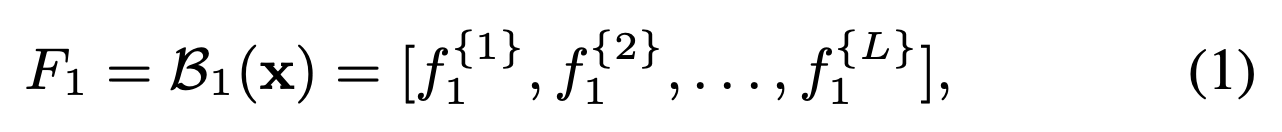 $F_1$을 추출한다.$L$은 #stages를 denotes (i.e., #multi-scale features)
  그리고 나서, router $R$은 $F_1$을 입력받아서 difficulty score $\phi \in (0, 1)$을 predict한다.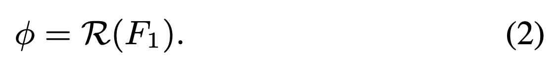일반적으로 말할 때,
  일반적으로, "easy" image는 첫 번째 backbone에서 exit되고,
  "hard" image는 추가 processing이 필요하다.
  구체적으로,
  router가 input image를 "easy" image로 분류하면,
  이어지는 neck and head $D_1$은 detection results $y$를 output한다.
  반면에,
  router가 input image를 "hard" image로 분류하면,
  the multi-scale features는 $D_1$으로 바로 decoding되지 않고,
  두 번째 backbone에 의해 추가로 enhancement되어야 할 필요가 있다.
  구체적으로,
  multi-scale features $F_1$을 composite(복합) connection module $G$를 사용하여 $H$로 embedding시킨다.
  $G$는 CBNet의 DHLC이다.그리고 나서, input image $x$를 두 번째 backbone에 입력하고,
  두 번째 backbone의 feature를 강화하기 위해 $H$의 각 stage에서 해당 elements를 순차적으로 합산한다.
  그러면 detection results $y$는 두 번째 head and neck $D_2$에 의해 얻어진다.위 과정을 통해서,
  "easy" image는 only one backbone만 processed될 것이고,
  "hard" image는 two backbone에 processed될 것이다.
  이러한 architecture 통해 computation(i.e., speed)와 accuracy 사이의 trade-offs를 조절할 수 있다.

3.2. Adaptive router

• object detector에서 다양한 scale의 feature들은 서로 다른 역할을 한다.
  일반적으로,
  shallow layer의 feature는 strong spatial information and small receptive fields를 가지고 있어서
  주로 small object를 detect하는 데 사용된다.
  deep layer의 feature는 strong semantic information and large receptive fields를 가지고 있어서
  주로 large object를 detect하는 데 사용된다.
  이러한 속성은 image의 difficulty score를 predicting할 때 multi-scale information을 고려하는 것을 필수적이게 한다.
  이를 기반으로, 우리는 multi-scale features에 기반한 adaptive router를 설계했다.
  이는 dynamic detector에 대한 간단하지만 효과적인 decision-maker이다.

• squeeze-and-excitation(SE) module에 영감 받아,
  우리는 multi-scale features인 $F_1$을 독립적으로 pooling하고 이를 모두 concatenate한다.$P$는 global average pooling을 denote하고
  $C$는 channel-wise concatenation을 denote한다.
  이 operation을 통해, multi-scale features $F_1$을 dimension $d$인 vector $\tilde{F_1} \in \R^d$로 압축한다.
  그런 다음, 이 vector를 두 개의 learnable fc layers를 통해 difficulty score $\phi \in (0, 1)$로 mappting한다.$\delta$는 ReLU, $\sigma$는 Sigmoid activation function을 의미한다.
  그리고 $W_1, W_2, b_1, b_2$는 learnable parameter를 의미한다.
  [59]에 따라서, 우리는 첫 번째 fc layer에서 feature dimension을 $\lfloor \frac{d}{4} \rfloor$로 줄이고,
  두 번째 fc layer에서는 Sigmoid를 사용하여 predicted score를 생선한다.
  주목할 점은, 모든 multi-scale features를 pooling하기 때문에 router의 부담이 무시할 수 있을 정도로 작다는 것이다.

3.3. Optimization strategy

• 이 section에서는 위의 dynamic architecture에 대한 optimization strategy를 설명한다.
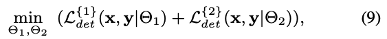
  먼저, 우리는 cascaded detectors를 jointly train하며, training objective는 다음과 같다.$x, y$는 각각 Input image와 ground truth를 나타낸다.
  $\Theta_i$는 detector $i$의 learnable parameters를 의미한다.
  $L^{\{i\}}_{det}$는 detector i에 대한 training loss를 의미한다 (e.g., bbox regression loss and classification loss)
  위의 training 단계 이후에, 두 개의 detectors는 objects를 detec할 수 있게 되고,
  trainng 이후에는 두 detector의 parameters인 $\Theta_1, \Theta_2$을 freeze한다.

• 그리고 나서,
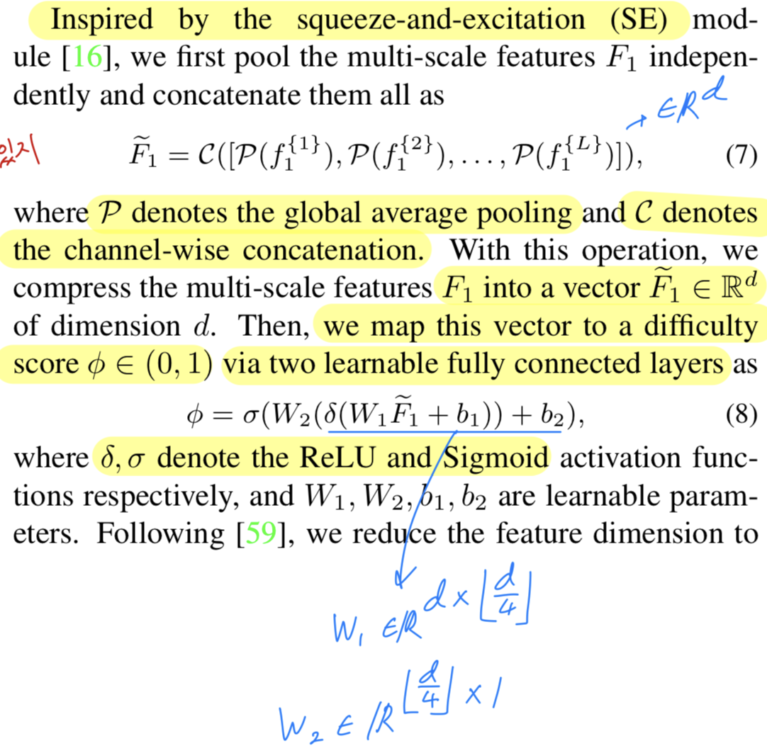
  우리는 adaptive router를 training하여 자동으로 image의 difficulty를 구분하도록 한다.
  여기서 router의 Parameters를 $\Theta_R$이라 하고
  predicted difficulty score은 Eq.(8)로부터 얻은 $\phi$이다.
  우리는 router가 "easy" images(i.e., with lower $\phi$)는 faster detector(i.e., the first detector)에 할당고
  "hard" images(i.e., with higher $\phi$)는 more accurate detector(i.e., the second detector)에 할당하기를 원한다.

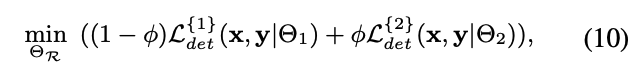
• 하지만 실제로 이를 구현하는 것은 단순하지 않다.
  아무런 제약 없이 바로 router를 optimize하면,
  router는 항상 lower training loss를 위해서 the most accurate detector를 선택하게 될 것이다.
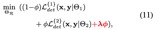
  게다가, 다음과 같이 만약 training objective에 hardware constraints를 단순히 더해준다면hyper parameter $\lambda$를 시행착오로 조정해야 하므로 막대한 workforce consumption(인력 소모)가 발생한다.
  위 문제를 극복하기 위해, 우리는 adaptive router에 대해 hyper parameter가 없는 optimization strategy를 제안한다.
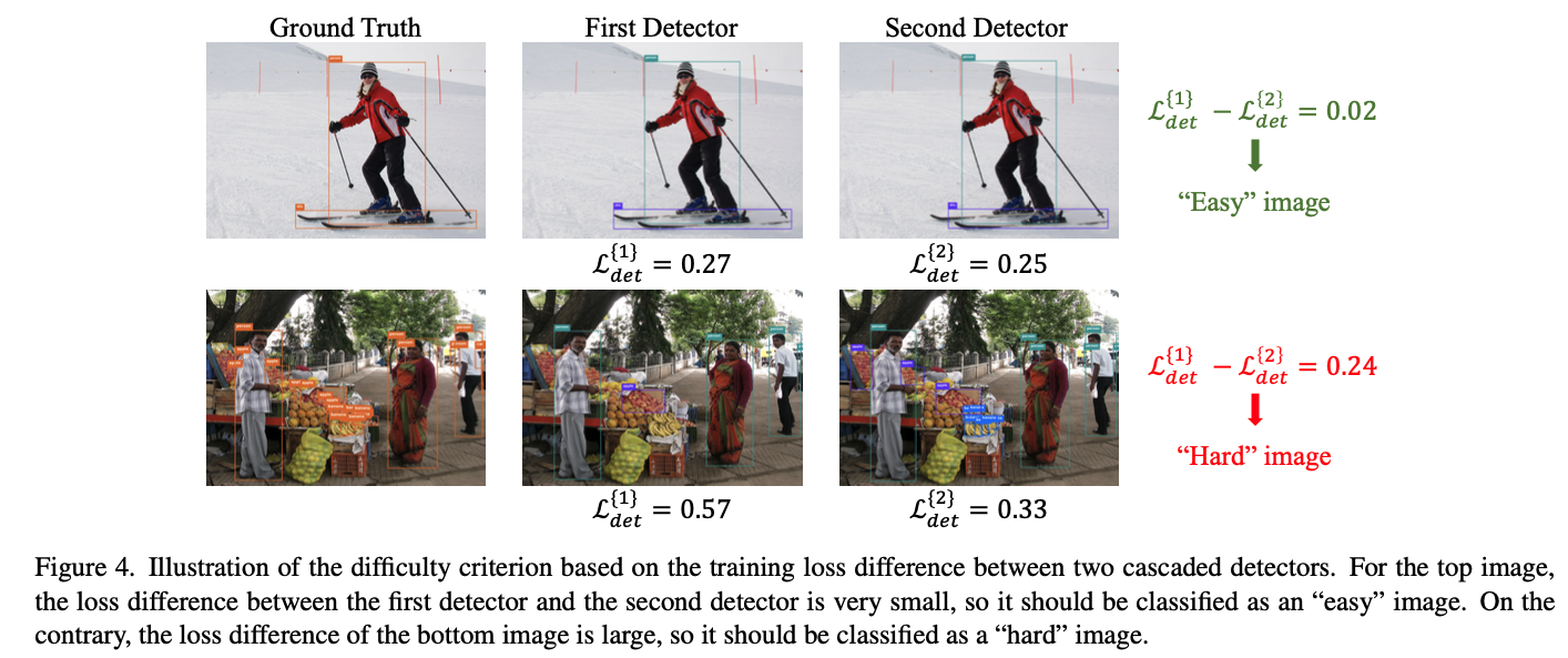
  먼저, Fig. 4.에서 보이는 것처럼, 두 detector의 image에 대한 loss difference를 기준으로 difficulty criterion을 정의한다.
  구체적으로,
  만약 image에 대한 두 detector의 loss difference가 충분히 작다면, 이 image는 "easy" image로 분류될 수 있다고 가정한다.
  반면, loss difference가 충분히 크다면, 이는 "hard" image로 분류되어야 한다.
  이상적으로는 balanced situation을 위해,
  우리는 모든 image의 절반은 first detector를 거치고, 나머지 절반은 second detector를 거치길 바란다.
  (내 생각 : 성능이 크게 떨어지지 않는다는 가정 하에 first detector만 거치는게 이상적이지 않은가?)
  이를 달성하기 위해, 두 detector의 loss를 균형 있게 하기 위한 adaptive offset을 도입하고, gradient descent를 통해 router를 optimize한다.
  실제로, 우리는 먼저 training set에서 first detector와 second detector의 training loss difference $\Delta$의 median(중앙값)을 계산했다.
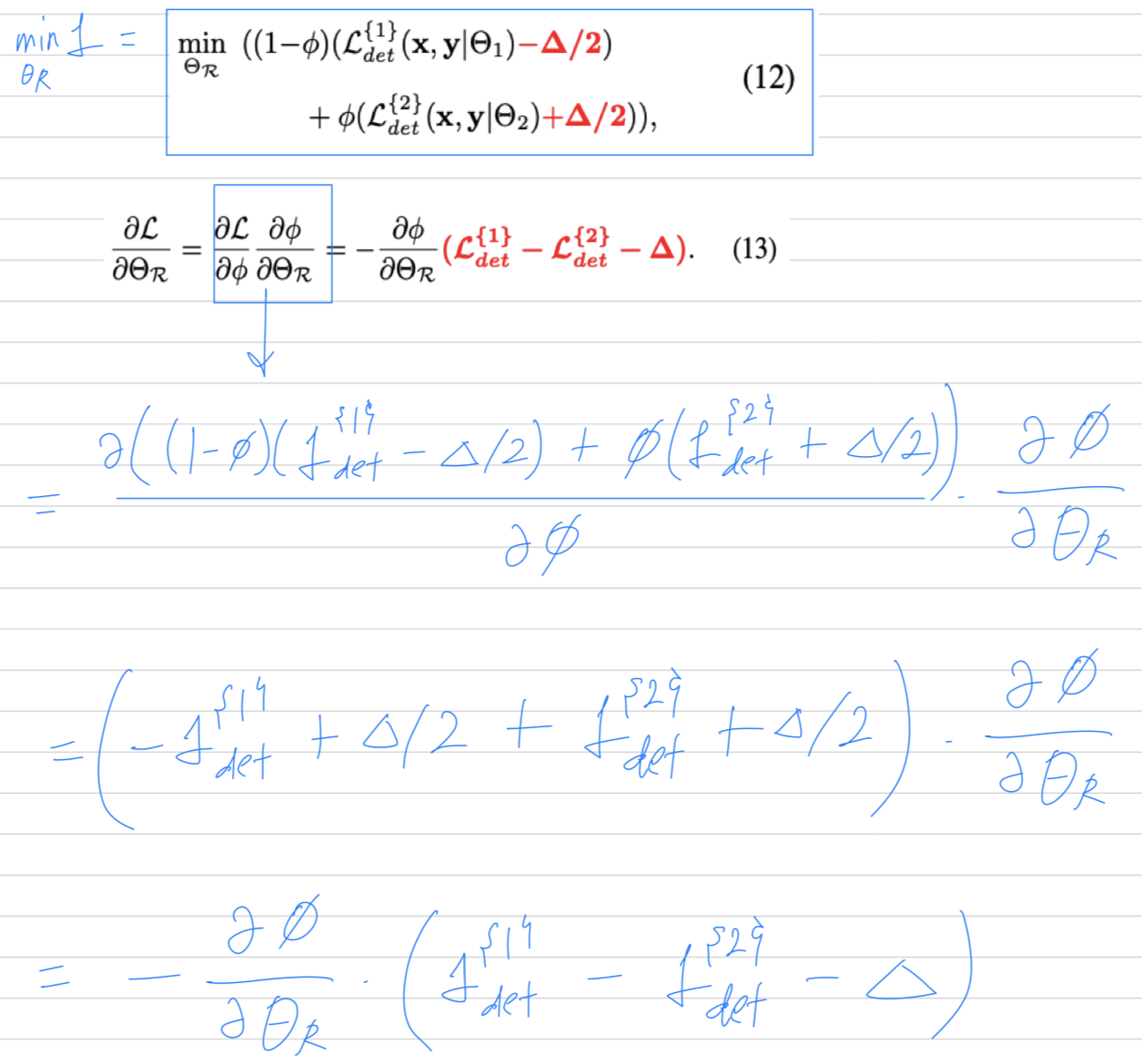
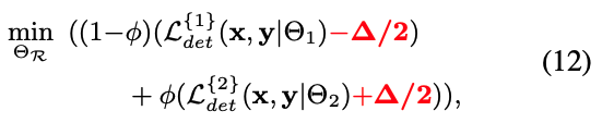
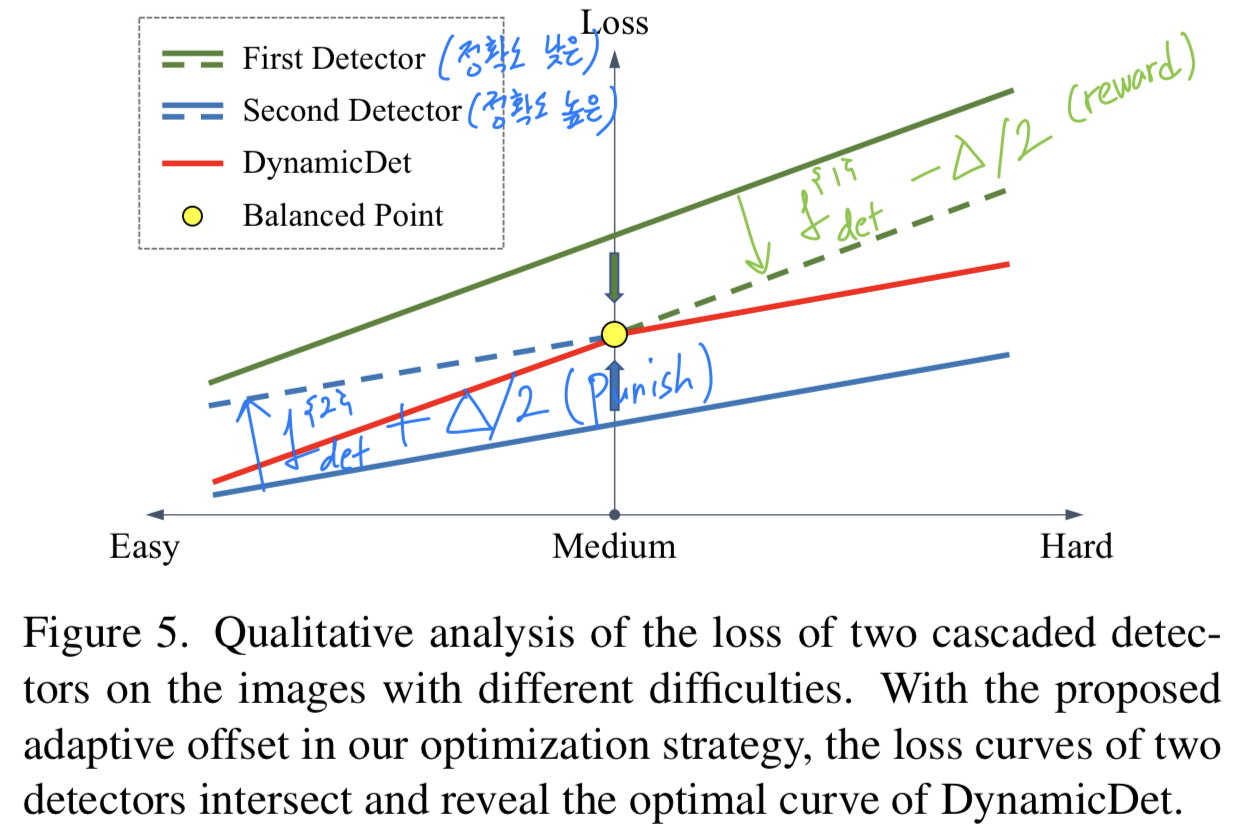
  그런 다음, router의 training objective는 다음과 같이 formulated될 수 있다.$\Delta/2$는 first detector에 reward와 second detector에 punish를 주기 위해 사용된다.Fig. 5.에서 보여지는 qualitative analysis에 따르면,
  이러한 reward and penalty 없이, second detector의 loss가 항상 first detector보다 작게 나타난다.
  하지만 reward and penalty를 적용하면, 두 loss curves는 intersect(교차)하며 optimal curve를 드러낸다.
  
  우리의 training objective는 difficulty score $\phi$를 통해
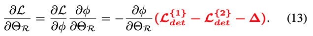
  router의 모든 parameters $\Theta_R$에 다음과 같은 gradient를 도입하여 adaptive router를 optimize하는 means(수단)을 제공한다."easy"와 "hard" images를 더 잘 구분하기 위해서,
  우리는 router의 optimization direction이 image의 difficulty, 즉 두 detector 간의 loss difference와 관련되기를 기대한다.
  분명히, Eq.(13)의 gradient는 이러한 기대를 가능하게 한다.

3.4. Variable-speed inference

• 우리는 only one dynamic detector로 variable-speed inference를 달성하기 위해 difficulty score thresholds를 결정하는 간단하고 효과적인 방법을 제안한다.
  구체적으로, 우리의adaptive router는 difficulty score를 예측하고, inference 중에 특정 threshold을 기준으로 어떤 detector를 사용할지 결정한다.
  따라서, 우리는 다양한 thresholds를 설정하여 서로 다른 accuracy-speed trade-offs를 달성할 수 있다.

• 먼저,
  우리는 validation set의 difficulty scores $S_{val}$을 계산한다.
  그리고 나서, 실제 필요(e.g. target latency)에 따라 router의 threshold를 설정할 수 있다.
  예를 들어,
  first detector의 latency를 $lat_1$,
  cascaded two detectors의 latency를 $lat_2$,
  target latency를 $lat_t$라고 하면,
  우리는 "hard" image의 maximum allowable proportion(최대 허용 비율) $k$를 다음과 같이 계산할 수 있다.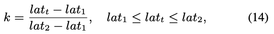그리고 threshold $\tau_{val}$은 다음과 같이 된다.여기서 $percentile(. , k)$은 $k$-번째 quantile(백분위수)를 계산함을 의미한다.
  주목할 점은, 이 threshold $\tau_{val}$는 validation set과 test set에 모두 robust하다는 것이다.
  이는 두 set가 independent and identically distributed(독립적이고 동일한 분포 i.e., i.i.d)를 따르기 때문이다.
  
  위의 전략을 기반으로, 하나의 dynamic detector는 single detector에서 double detector로의 accuracy-speed trade-offs를 직접적으로 다룰 수 있으며,
  이는 다양한 HW constraints 하에서 여러 detector를 redesigning하고 training하는 것을 피할 수 있게 한다.

---

4. Experiments

4.1. Experimental setups

• 우리는 COCO benchmark에 대해서 실험했다.
  모든 models은 118k training images, and tested on the 5k minival images and 20k test-dev images를 사용하여 test했다.
  우리는 YOLOv7 series model을 real-time detector baseline으로 선택했으며,
  Faster R-CNN과 Mask R-CNN을 two-stage detector baselines으로 사용했다.
  모든 dynamic detector들은 해당 baseline model들과 same hyper-parameters로 train되어졌다.

• 각 dynamic detector의 easy-hard proportion을 간략하게 나타내기 위해,
  예를 들어 "Dy-YOLOv7-X/10"은 dynamic YOLOv7-X model에서 10%의 image가 "hard" image로 분류되고 나머지 90%는 "easy" image로 분류됨을 의미한다.