Abstract

• ImageNet LSVRC-2010 contest에서 제공하는 $1.2 million$ high-resolution image를 1000개의 class로 classification하기 위한 Deep CNN을 학습시켰다.

• The neural network, which has $60 million$ parameters and $650,000$ neurons,
  consists of five convolutional layers, some of which are followed by max-pooling layers, and three FC layers with a final 1000-way softmax.

• To make training faster,
  we used non-saturating neurons and a very efficient GPU implementation of the convolution operation
  ➡️ non-saturating neurons 이해를 위해 참고한 사이트 : https://stats.stackexchange.com/questions/174295/what-does-the-term-saturating-nonlinearities-mean

• To reduce overfitting in the fully-connected layers
  we employed a recently-developed regularization method called "dropout”

---

1. Introduction

• Simple recognition task들은 dataset 사이즈가 작아도 잘 수행될 수 있다.
  예시로, MNIST digit-recognition task는 human performance에 근접한 0.3% 미만의 error rate를 보여준다.

• 하지만 현실로 다양하게 존재하는 object들을 학습시키기 위해, much larger training sets을 사용해야 한다.
  실제로 수 백만 개의 image가 label된 dataset을 수집하는 것은 최근에서야 가능해졌다.

  • LabelMe(https://github.com/wkentaro/labelme) : Labelme is a graphical image annotation tool
  • ImageNet(https://www.image-net.org/) : ImageNet is an image database organized according to the WordNet hierarchy (currently only the nouns(명사))
    • WordNet : WordNet is a large lexical database of English. (Nouns, verbs, adjectives and adverbs)

• CNN capacity는 그것의 depth와 breadth (깊이와 넓이)를 조정함으로써 control되어질 수 있다.
  CNN은 또한 image의 특성에 대해 강력하고 정확한 가정을 한다.
  그러므로 비슷한 size의 layer를 갖고 있는 standard feedforward neural network와 비교하여,
  CNN은 더욱 적은 connection과 parameter를 갖고 있고, train 시키기에 더욱 쉽다.

• 운이 좋게, current GPUs는 2D convolution에 매우 최적화되었고, CNN training을 시키는 데에 충분하다.
  또한 ImageNet과 같은 dataset은 overfitting 없는 model로 훈련시키기에 충분한 양의 labeled examples이 있다.

• Section 3 : 우리는 highly-optimized GPU implementation of 2D convolution을 사용했다.
  그리고 performance를 향상시키고 training time을 감소시키는 새롭고 특이한 방법들을 사용했다.

• Section 4 : 우리의 network는 1.2M개의 labeled training examples을 갖고도 심각한 overfitting 문제를 겪었다.
  overfitting을 예방하기 위해 몇가지 effective techniques들을 사용했다.

• Our final network contains five convolutional and three fully-connected layers.
  그리고 이러한 depth는 매우 중요한 듯 보인다.
  우리는 model의 parameter 중 1% 이상도 갖지 않는 convolutional layer를 제거했더니 performance가 떨어지는 것을 발견했다.

• network의 size는 현재 GPU에서 사용가능한 memory 양에 의해 제한되어진다.
  Our network takes between 5 and 6 days to train on two GTX 580 3GB GPUs.

---

2. The Dataset

• ImageNet is a dataset of over $15M$ labeled high-resolution images belonging to roughly 22,000 categories.
  The images were collected from the web and labeled by human labelers using Amazon's Mechanical Turk crowd-sourcing tool.
  (https://blog.mturk.com/tutorial-how-to-label-thousands-of-images-using-the-crowd-bea164ccbefc)

• Starting in 2010, as part of the Pascal Visual Object Challenge,
  an anuual competition called the ImageNet Large-Scale Visual Recognition Challenge(ILSVRC) has been held.
  ILSVRC uses a subset of ImageNet with rougly 1000 images in each of 1000 categories.
  https://image-net.org/challenges/LSVRC/2010/

• ImageNet consists of variable-resolution images, while our system requires a constant input dimensionality.
  Therefore, we down-sampled the images to a fixed resolution of 256 x 256.

  • Given a rectangular image,
    we first rescaled the image such that the shorter side was of length 256,
    and then cropped out the central 256 x 256 patch from the resulting image.
    We did not pre-process the images in any other way, except for subtracting the mean activity.

---

3. The Architecture

ReLU Nonlinearlity

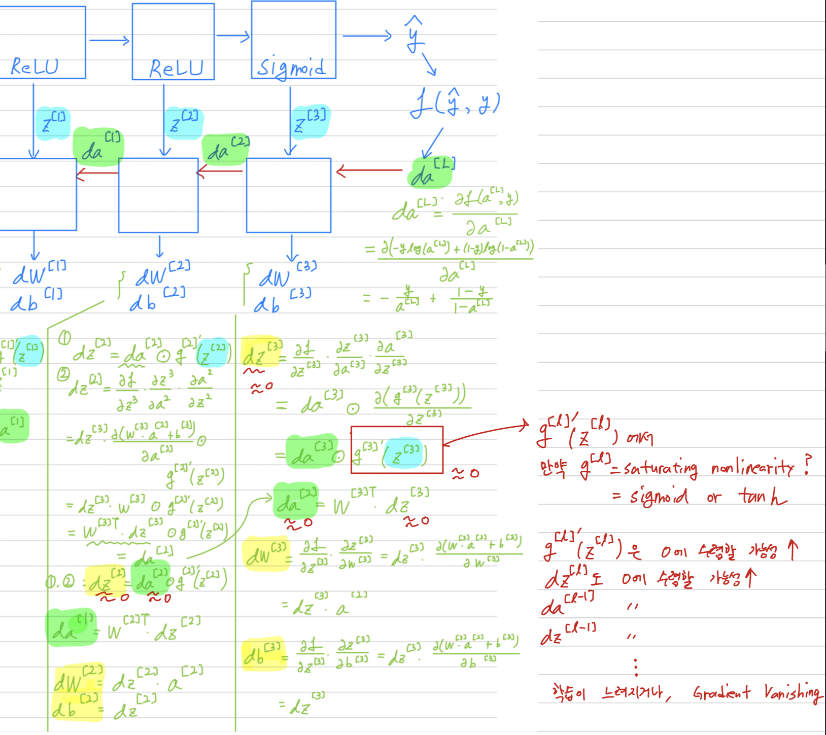
• The standard way to model a neuron's output $f$ as a function of its input $x$ is with
  $f(x) = tanh(x)$ or $f(x)=(1+e^{-x})^{-1}$.
  These saturating nonlinearities are much slower than the non-saturating nonlinearity $f(x)=max(0, x)$

• Following V. Nair and G. E. Hinton. Rectified linear units improve restricted boltzmann machines,
  we refer to neurons with this nonlinearity as Rectified Linear Units(ReLUs) train several times faster than their equivalents with $tanh$ units.
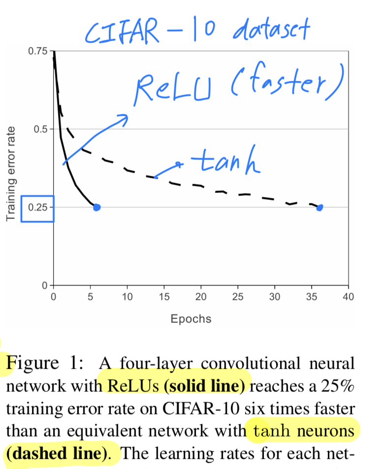  This is demonstrated in Figure 1, which shows the number of iterations required to reach $25$% training error on the CIFAR-10 dataset for a particular four-layer convolutional network.
  This plot shows that "traditional saturating neuron models($sigmoid$ or $tanh$)를 사용하여 large neural network를 실험할 수 없을 것이다."
  

• 이번 dataset에서 가장 주요한 점은 preventing ovefitting이다(아마도 test set에 대하여 순위를 측정하는 대회였기 때문?).
  ReLU를 사용함으로써 training set에 fit하는 것을 더욱 가속화할 수 있었기 때문에 ovefitting을 방지할 수 있었고,
  이러한 faster learning은 large dataset을 train하는 model의 performance에 좋은 영향을 미친다.

Training on Multiple GPUs

• https://www.techpowerup.com/gpu-specs/evga-gtx-580-3-gb.b1543

• A single GTX 580 GPU has only 3GB of memory.
  하나의 GPU로 약 $1.2M$개의 training examples를 학습시키기 힘들었다.
  그래서 we spread the net across two GPUs.
  Current GPUs are particularly well-suited to cross-GPU parallelization,
  as they are able to read from and write to one another's memory directly
  , without going through host machine memory.

• The parallelization scheme that we employ essentially puts half of the kernels(or neurons) on each GPU,
  (중요하게 생각했던 GPU parallelization scheme는 kernel을 반으로 나누어 각각 하나의 GPU에 할당하는 것이었다.)
  which additional trick : the GPUs communicate only in certain layers.
  For example, the kernels of layer 3 take input from all kernel maps in the layer 2.
  However kernels in layer 4 take input only from those kernel maps in layer 3 which reside on the same GPU.
  ➡️ Choosing the pattern of connectivity is a problem for cross-validation,
  but this allows us to precisely tune the amount of communication until it is an acceptable fraction of the amount of computation.

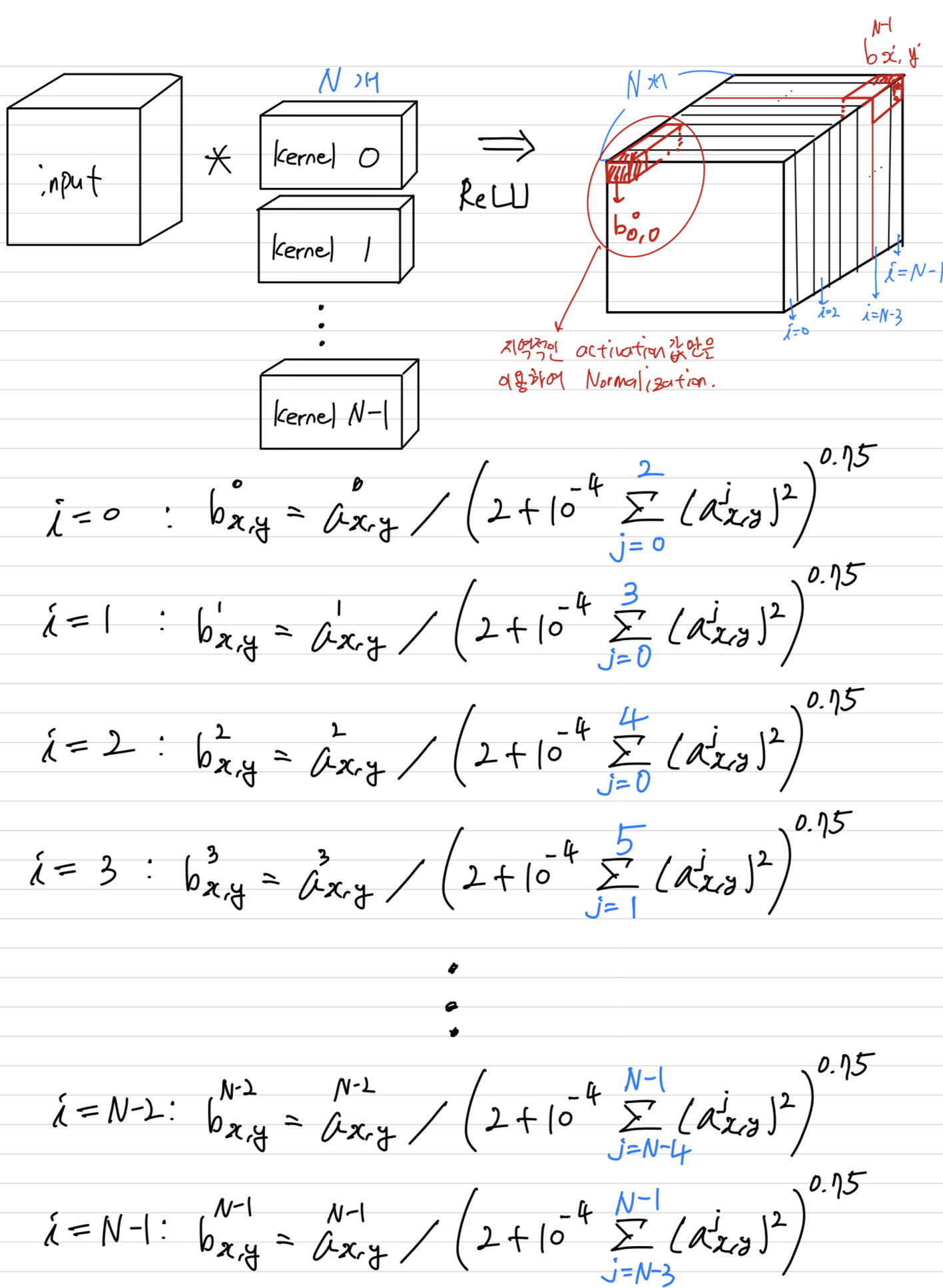
Local Response Normalization

• We find that the following local normalization scheme aids generalization.
  

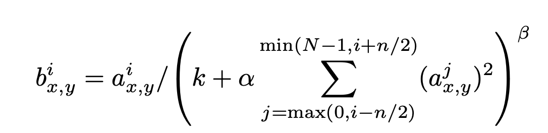
• Denoting

  • $N$ : the total number of kernels in the layer.
  • $a^i_{x, y}$ : the activity of a neuron computed by applying kernel $i$ at position $(x, y)$ and then applying the ReLU nonlinearity
  • $b^i_{x, y}$ : response-normalized activity is given by the expression
  • $k, n, \alpha, \beta$ : hyper-parameters
    • $k=2$
    • $n=5$ : the sum runs onver $n$ "adjacent" kernel maps at the same spatial position.
    • $\alpha=10^{-4}$
    • $\beta=0.75$

• 이해하기 위해 그린 Local Response Noramlization
  This sort of response normalization implements a form of lateral inhibition inspired by the type found in real neurons,
  creating competition for big activities amongst neuron outputs computed using different kernels.
  ($n$으로 얼마나 많은 주위 Kernel값을 볼 것인지 조절할 수 있는듯.)
  (여기서는 $n=5$인 상수이고, 2로 나눠주었기 때문에
  만약 내가 3번 kernel이라면, 3-2=1 kernel ~ 3+2=5 kernel의 값으로 LRN을 진행한다.
  $\Sigma$에 min, max가 있는 이유는 kernel은 0~(N-1)의 양수의 index를 갖기 때문에 음수가 되는 것을 막기 위해 사용되었다.)
  그리고 mean값을 빼주는 과정이 없기 때문에 일반적인 Normalization보다는 값이 클 것이므로,
  더 정확히는 brightness normalization이라고 할 것이다.
  ➡️ Local Response Normalization을 사용한 의도는?
  논문에서 실제 뇌세포에서 일어나는 생리적 현상에서 영감을 받아 구현하였다고 한다.
  (참고 : https://www.youtube.com/watch?v=40Gdctb55BY)
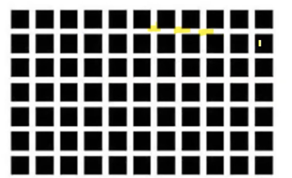  위에서 보면,
  강한 뉴런의 활성화인 검은색 주변에 있는 흰 선은 밝게 보이지만,
  흰 선 주변에 있는 흰 선을 보면, 보다 어둡게 보여서 회색으로 보이는 착시가 나타난다.
  
  이렇게 주변 값들 보다 강하게 활성화한 뉴런이 근처 다른 뉴런의 활성화를 억제시키기 위하여 LRN을 사용했다.
  ➡️ (나의 의견) : 여기서 한 방법은 kernel 간 Local Response Normalization이었는데,
  kernel 내에서 Local Response Normalization을 사용한다면 더욱 효과적일 것 같다.
  왜냐하면 서로 연관이 없는 kernel끼리 normalization할 때, 이용되는 activation값도 연관이 없을 것이기 때문에 하나의 kernel 내의 activation값끼리 normalization하는 것이 더욱 효과가 있을 것 같다.

• LRN을 사용해서 top-1 and top-5 error rate가 각각 1.4% and 1.2% 줄어들었다.

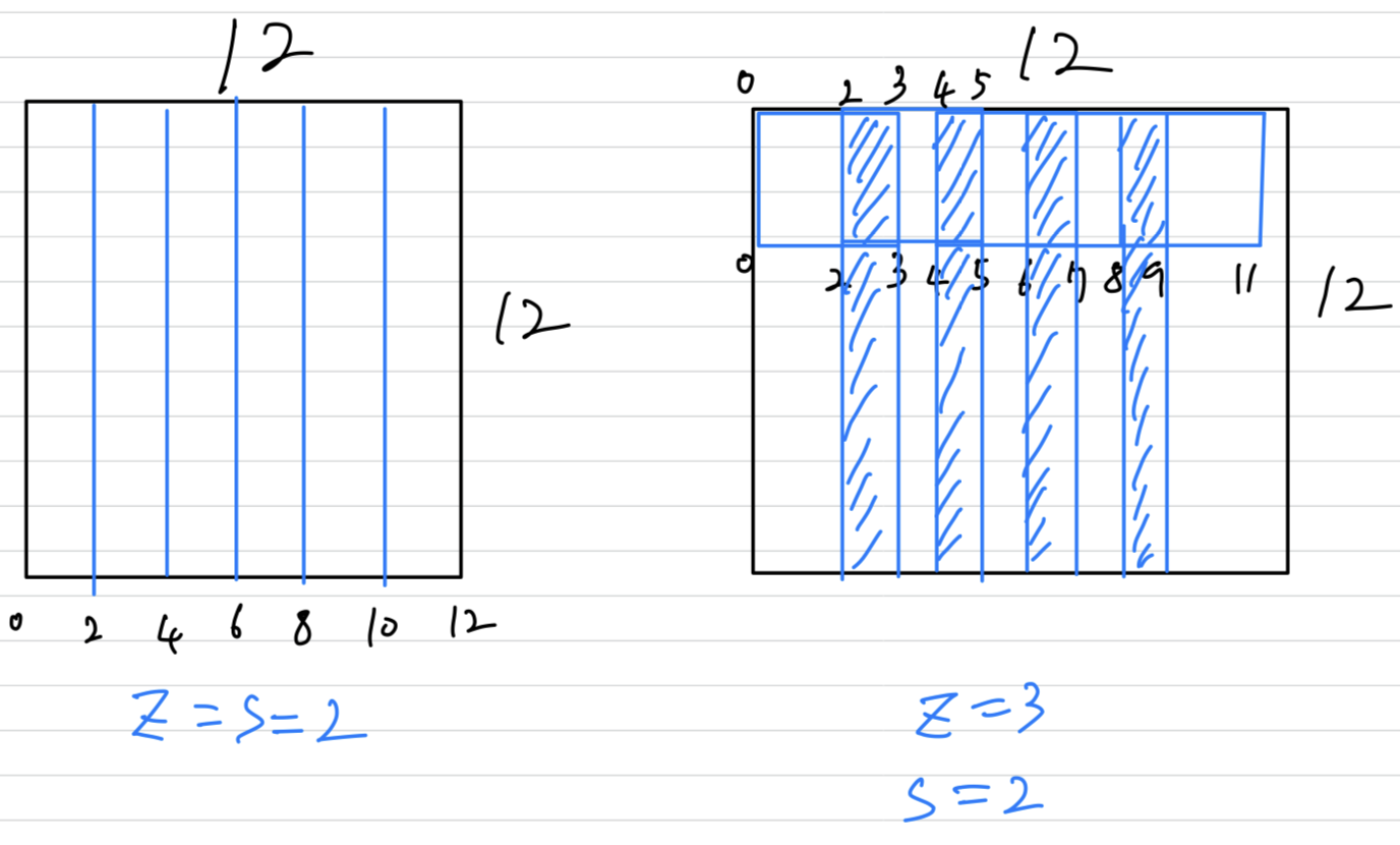
Overlapping Pooling

• This scheme(Overlapping Pooling, $s=2$, $z=3$) reduces the top-1 and top-5 error rates by 0.4% and 0.3%, respectively,
  as compared with the non-overlapping scheme $s=2$, $z=2$.
  
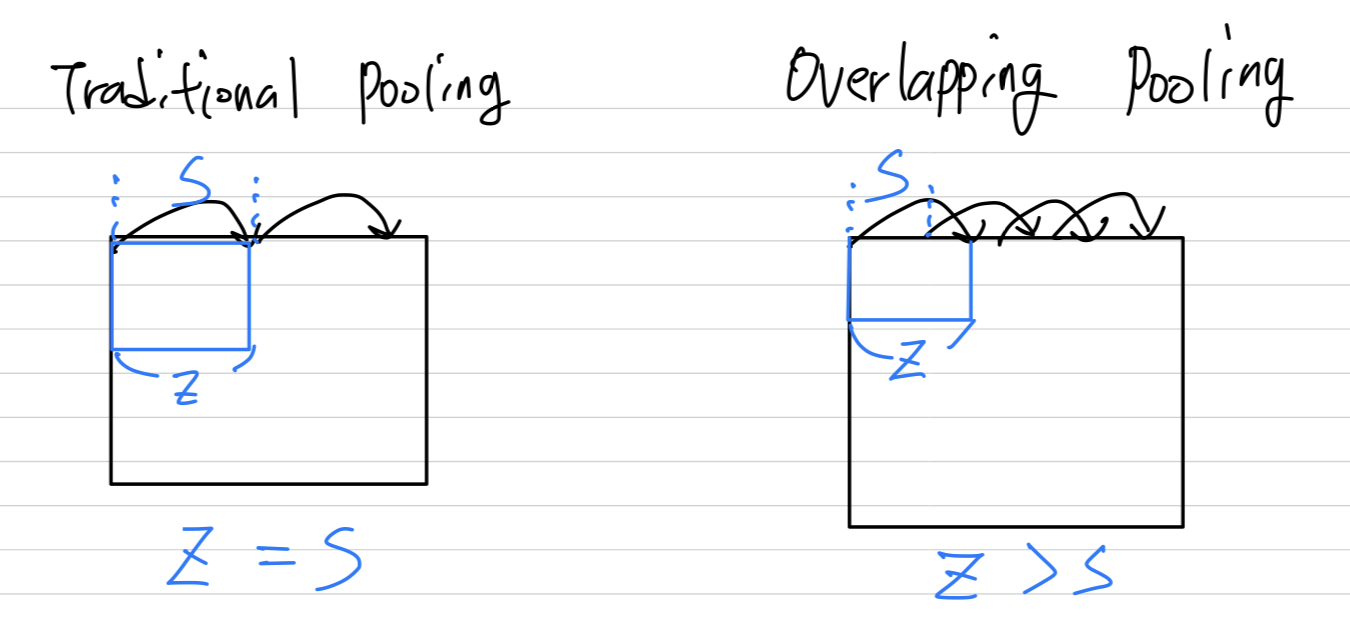
  We generally observe during training that models with overlapping pooling find it slightly more difficult to overfit.
  ➡️ 왜 overlapping pooling을 사용한 것이 정확도가 조금 더 높게 나왔을까?
  (나의 의견)
  모서리에 있지 않은 값들은 pooling에 중복되어 사용되어지기 때문에
  주변 값들과의 상관관계를 보다 많이 비교하게 된다.
  더욱 더 많은 비교를 통해 max값을 뽑아내는 것이므로 output에는 보다 다양한 feature들이 뽑힐 것이므로
  performance에 아주 조금은 도움이 될 것 같다.

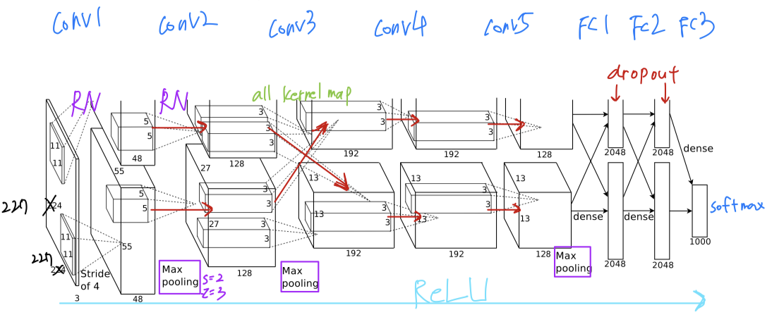
Overal Architecture

• The net contains eight layers with weights;
  the first five are convolutional and the remaining three are fully-connected.
  The output of the last fully-connected layer is fed to a 1000-way softmax.
  

• The kernels of 2, 4, 5 convolutional layers are connected only to those kernel maps in the previous layer which reside on the same GPU.

• The kernels of 3 convolutional layer are connected to all kernel maps in the previous layer.
  = The GPUs communicate only at certain layers.
  ➡️ 왜 3번째 layer만 모든 neuron이 연결되게 했을까?
  

• Response-normalization layers follow the 1 and 2 convolutional layers.
  Max-pooling layers follow both response-normliazation layers as well as the 5 convolutional layer.

• The ReLU non-linearity is applied to the output of every convolutional and fully-connected layer.

Self Dimension Checking

• 다음은 직접 dimension을 계산해본 그림이다.
  
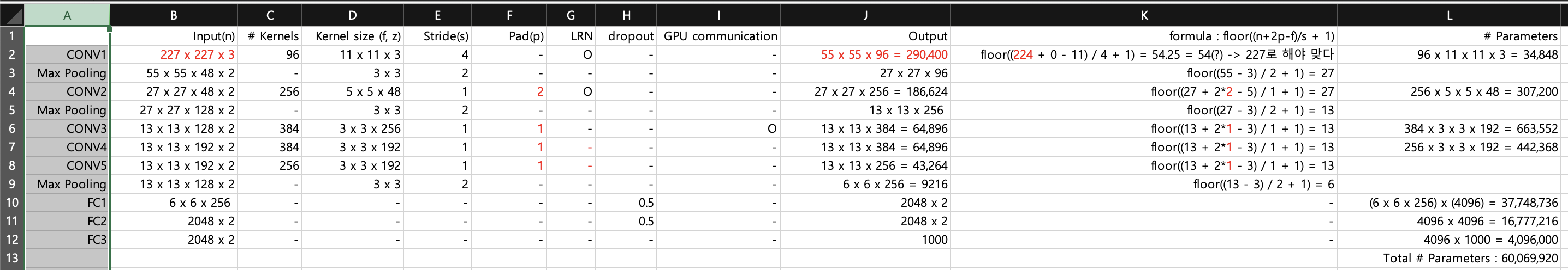
  • 특이점 1 :
    논문에서는 input image가 224 x 224 x 3으로 되어있지만,
    dimension을 직접 구해봤을 때, output volume의 width와 height는 floor(54.25)=54로
    다음 Convolutional layer 2의 input으로 55 x 55 x 96의 dimesion과 맞지 않게 된다.
    따라서 input image의 width와 height는 최소 227이 되어야 한다.
    (+ 저자는 추후에 227인데 224로 오기하였다고 말한 바가 있다)
  • 특이점 2 :
    본 논문에서는 Padding에 대한 정보가 없었다.
    하지만 CONV2, CONV3, CONV4, CONV5의 dimension을 일치시키기 위해서는
    각각 2, 1, 1, 1의 padding이 필요하다.
    따라서 논문에서는 padding이 언급되지 않았지만, 실제로는 padding을 사용했을 것으로 추측된다.
    (https://learnopencv.com/understanding-alexnet/)

---

4. Reducing Overfitting

• AlexNet architecture has 약 $60M$ parameters.
  1000개의 class를 분류하기 위해서 10bit($2^{10}=1024$)에 mapping 하는 것에도 불구하고
  약 $60M$개의 parameters를 학습시키는 것은 overfitting을 유발한다고 밝혀졌다.
  따라서 overfitting을 줄이기 위한 two primary ways를 설명하겠다.

Data Augmentation

• The easiest and most common method to reduce overfitting on image data is to artificially enlarge the dataset using label-preserving transformations.
• The transformed images are generated in Python code on the CPU while the GPU is training on the previous batch of images.

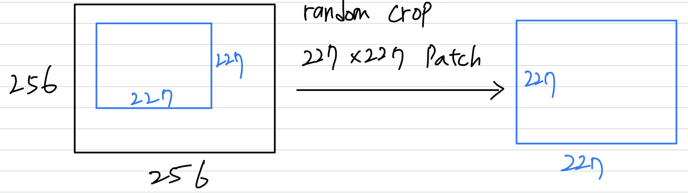
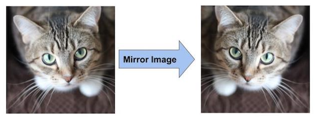
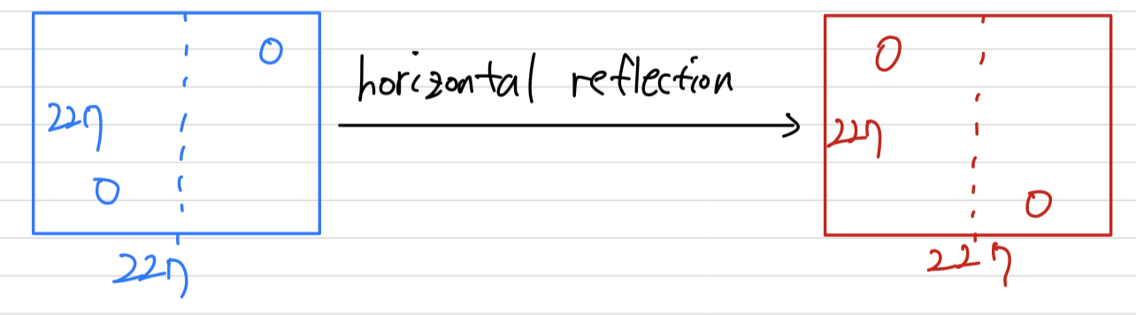
1. The first form of data augmentation consists of generating image translation and horizontal reflections.
   (image crop, y축 대칭)
   We do this by extracting random 227 x 277 patches(and their horizontal reflections) from the 256 x 256 images and training our network on these extracted patches(227 x 227 x 3).
   
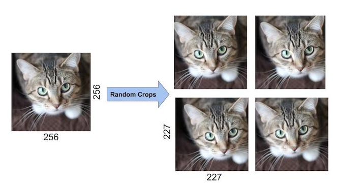
   At test time, the network makes a prediction by extracting five 227 x 227 patches(the four corner patches and the center patch) as well as their horizontal reflections(hence then patches in all),
   and averaging the predictions made by the ntwork's softmax layer on the ten patches.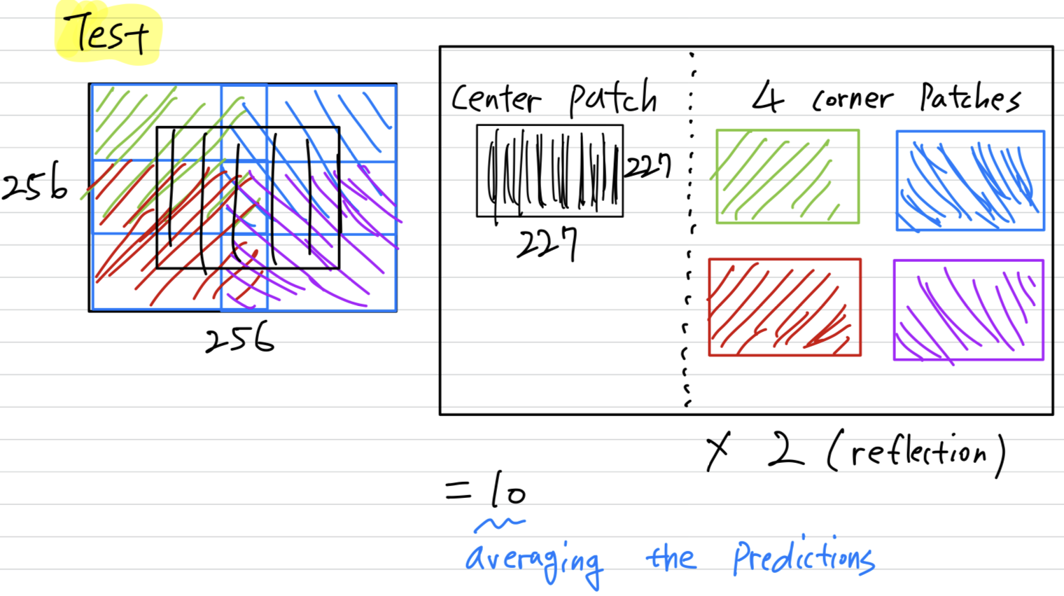

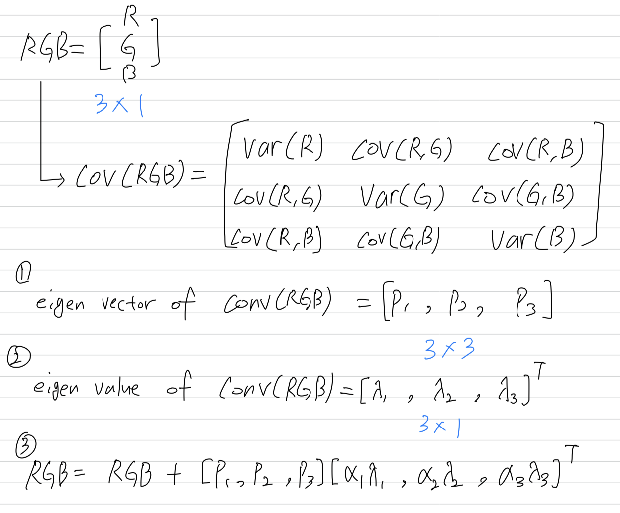
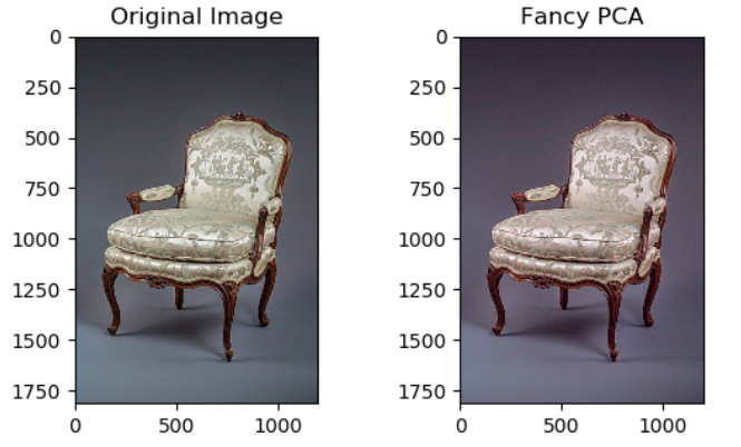
2. The second form of data augmentation consists of altering the intensities of the RGB channels in training images.
   Specifically, we perform PCA on the set of RGB pixel values throughout the ImageNet training set.
   = PCA Color Augmentation = Fancy PCA
   To each training image, we add multiples of the found principal components, with magnitudes proportional to the correspoinding eigenvalues times a random variable drawn from a Gaussian with mean $0$ and standard deviation $0.1$.
   Therefore to each RGB image pixel $I_{xy} = [I^R_{xy}, I^G_{xy}, I^B_{xy},]^T$ we add the following quantity :
   $[p1, p2, p3][\alpha_1\lambda_1, \alpha_2\lambda_2, \alpha_3\lambda_3]^T$ where $p_i$ and $\lambda_i$ are $i$th eigenvector and eigenvalue
   of the 3 x 3 covariance matrix of RGB pixel values, respectively, and $\alpha_i$ is random variable(mean 0, std dev 0.1).
   (https://pixelatedbrian.github.io/2018-04-29-fancy_pca/)

Dropout

• There is a very efficient version of model combination that only costs about a factor of two during training.
  The recently-introduced technique, called "dropout", cosists of setting to zero the output of each hidden neuron with probability 0.5.
  The neurons which are "dropped out" in this way do not contribute to the forward pass and do not participate in back-propagation.
  This technique reduces complex co-adaptations of neurons, since a neuron cannot rely on the presence of particular other neurons.
  At test time, we use all the neurons but multiply their outputs by 0.5, which is a reasonable approximation to taking the geometric mean of the predictive distributions produced by the exponentially-many dropout networks.
  
  we use dropout in the first two fully-connected layers.
  ➡️ (나의 생각)특정 neuron의 영향력을 낮춤으로써 그 외의 다른 neuron들이 학습에 참여가 낮거나 느려지는 문제를 개선한다.

---

5. Details of learning

• Stochastic Gradient Descent with a batch size of 128 examples.
  (SGD는 example 하나에 대해서 iteration 돌리는 것 아니었나?
  왜 128개의 batch size를 정하지?
  이러면 mini batch gradient descent 아닌가?)

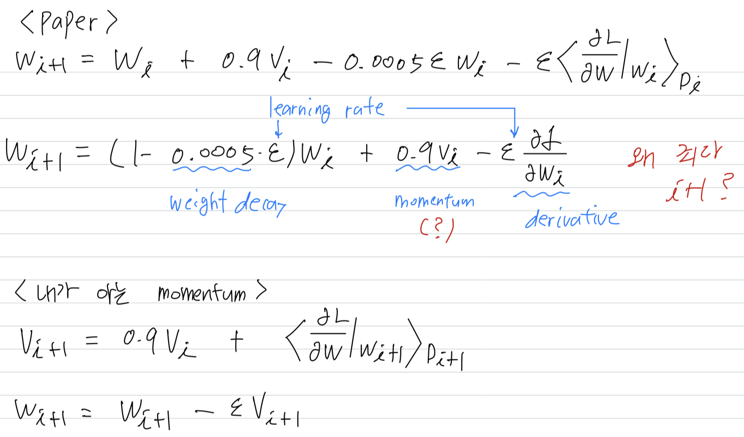
• momentum 0.9

• weight decay 0.0005
  ➡️ weight decay here is not merely a regularizer : it reduces the model's training error.

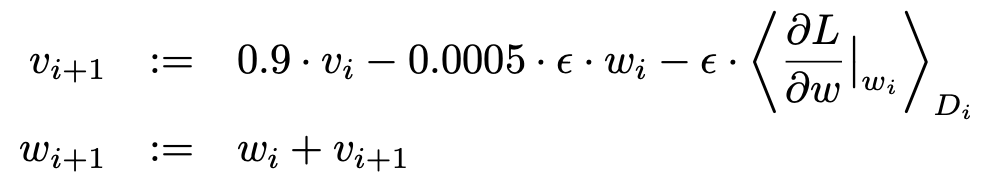
• The update rule for weigth $w$ was
  

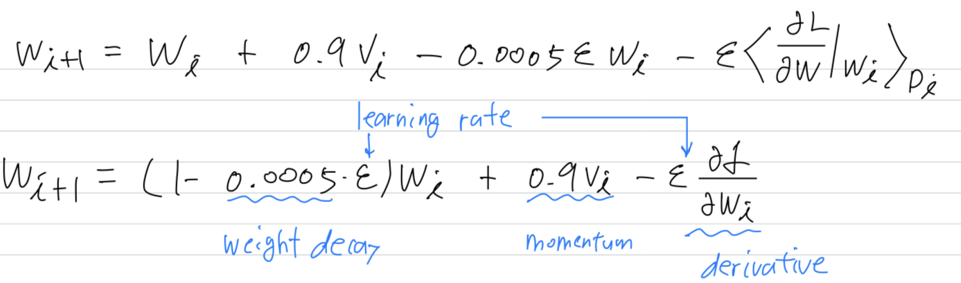
  • $i$ : interation index
  • $v$ : momentum variable
  • $\epsilon$ : learning rate
  • $<\frac{\partial L}{\partial w} | _{w_i}>_{D_i}$ : the average over the $i$th batch $D_i$, of the derivatives of the objective with respect to $w$, evaluated at $w_i$.

• Initial Weight : zero-mean Gaussian distribution with standard deviation 0.01.

• Initial Bias :
  2, 4, 5 convolutional layers, as well FC hidden layers, with the constant 1.
  remaining layers with the constant 0.

• Initial Learning Rate : 0.01
  The heurisitc which we followed was to divide the learning rate by 10 when the validation error rate improving with the current learning rate.
  (validation error rate가 현재의 learning rate로 개선되는 것이 멈췄을 때 10으로 divide하는 것
  ➡️ (나의 생각)overshooting으로 더 이상 global minimum에 접근하지 못하는 것이라 생각해서 learning rate를 더 작게 만들어준 것 같다.)

• Epoch : 90

---

6. Results

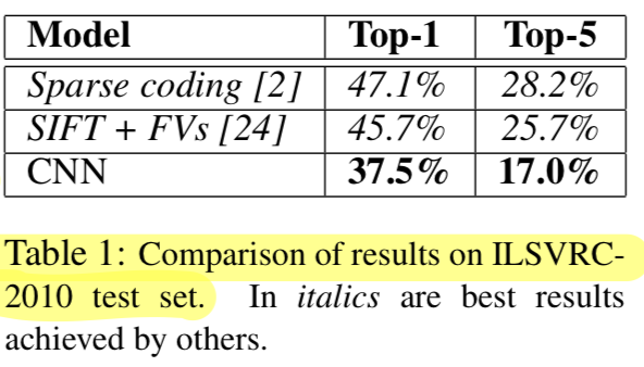
• Our results on ILSVRC-2010 are summarized Table 1.
  Our network achieves top-1 and top-5 test set error rates of $37.5$% and $17.0$%.
  The best performance achieved during the ILSVRC-2010 competition was 47.1% and 28.2%.
  (나는 지금까지 AlexNet이 ILSVRC-2010 우승팀인줄 알았는데 아니었음...
  AlexNet은 ILSVRC-2010 대회가 끝난 뒤 개발된 model이었음)
  

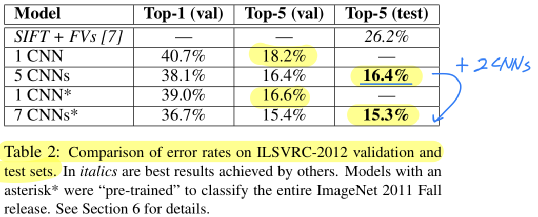
• We also entered our model in the ILSVRC-2012 competition.
  Since the ILSVRC-2012 test set labels are not publicly avaiable,
  we cannot report test error rates for all the models that we tried.
  We use validation and test error rates interchangeably because in our experience they do not differ by more than 0.1%(Table 2)
  
  Averaging the predictions of five similar CNNs gives an error rate of 16.4%
  Training one CNN, to classify the entire ImageNet Fall 2011 release, and then "fine-tuning" it on ILSVRC-2012 gives an error rate of 16.6%.
  
  Averaging the predictions of two CNNs that were pre-trained on the entire Fall 2011 release with the aforementioned five CNNs gives an error rate of 15.3%.

Qualitative Evaluations

• Figure 3 shows the convolutional kernels learned by the network's two data-connected layers.
  
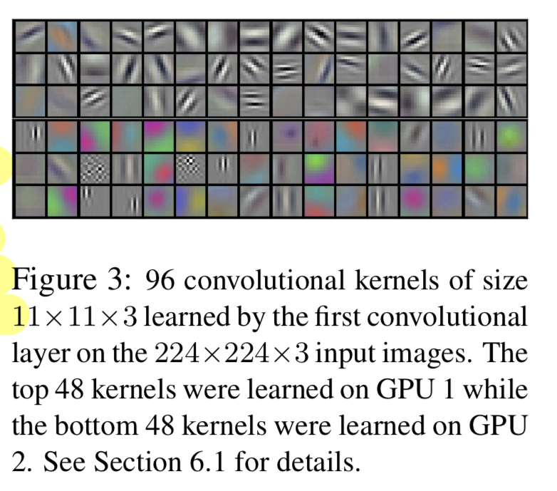
  두 개의 GPU는 각각 서로 다른 것을 학습한다고 한다.
  예를 들어, GPU1은 frequency, orientation과 관련된 kernel을 학습하고,
  GPU2는 color를 중점으로 학습한다고 한다.

• In the left panel of Figure 4 we qualitatively assess what the network has learned by computing its top-5 predictions on eight test images.
  

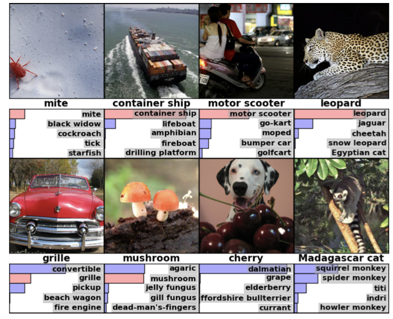
  • mite(진드기)가 image의 가운데에 있지 않는데도 불구하고 잘 분류되는 것을 알 수 있다.
  • 또한 고양이과의 종류로 잘 알려진 leopard(표범)도 잘 분류되고 있다.
  • grille, cherry와 같이 애매모호한 것도 있긴 하다.

• 이처럼 시각화하여 정보를 알 수 있는 또 다른 방법은 4096-dimensional hidden layer의 activations값을 고려하는 것이다.
  만약 두 image의 Euclidean separation값이 작다면, 두 image는 비슷하다고 말할 수 있다.
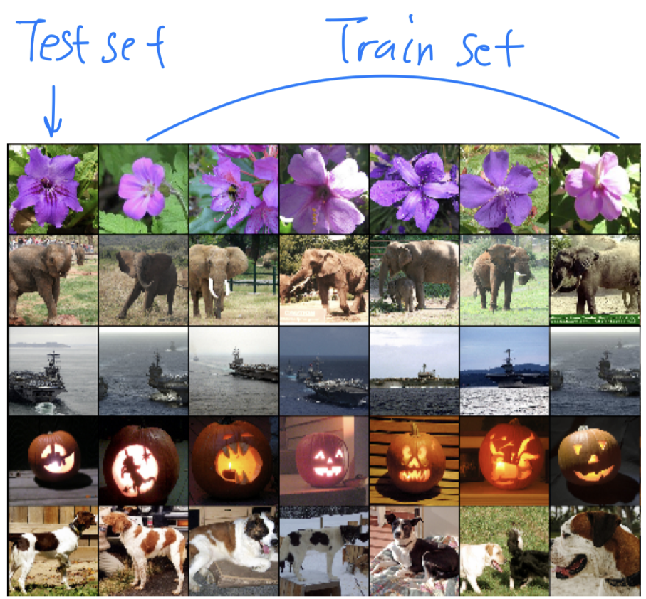  예를 들어 위의 5개의 test set image와 6개의 train set image들이 있는데,
  이는 Euclidean separation값이 비슷한 image들을 모아 비교한 것이다.
  
  이처럼 두 4096-dimensional vector 사이의 Euclidean distance를 계산하는 것은 매우 비효율적이지만,
  이러한 vector를 short binary codes로 auto-encoder로 압축하여 traning함으로써 효율적일 수 있다. (?)
  이렇게 하면 raw pixel에 auto encoder를 적용하는 것보다 훨씬 나은 image retrieval method가 될 수 있다.
  왜냐하면 image label을 사용하지 않으므로 의미론적으로 유사한지 여부에 상관없이 유사한 패턴의 edge가 있는 image를 찾는 경향이 있게 된다.
  (https://www.cs.toronto.edu/~hinton/absps/esann-deep-final.pdf)

---

7. Discussion

• It is notable that our network's performance degrades if a single convolutional layer is removed.
  For example, removing any of the middle layers results in a loss of about 2% for the top-1 performance of the network.
  So the depth really is important for achieving our results.

• We did not use any unsupervised pre-training even though we expect that it will help.
  Thus far, our results have improved as we have made our network larger and trained it longer
  but still have many orders of magnitude to go in order to match the infero-temporal pathway of the human visual system.
  (인간의 시각 체계의 infero-temproal pathway를 만족시키기에 아직 멀었다.)
  Ultimately we would like to use very large and deep convolutional nets on video sequences where the temporal structure provides very helpful information that is missing or far less obvious in static images.

---

궁금한 점

• Two GPUs

  • 왜 GPU를 conv2-conv3에서만 communication하게 한 것일까? 효과는? 안했다면?
  • columnar CNN이란?
  • "Choosing the pattern of connectivity is a problem for cross-validation,
    but this allows us to precisely tune the amount of communication until it is an acceptable fraction of the amount of computation."
    ➡️ 해석, 의미를 잘 모르겠다.
    ➡️ 나의 해석 : con2-conv3에서만 두 GPU가 통신하도록 하는 이러한 pattern이 cross-validation에 문제를 미칠 수 있다.
    하지만 이러한 pattern을 통해서 GPU가 할 수 있는 computation양을 잘 조절할 수 있다.

• Local Response Normalization이 왜 효과가 있었을까?

• 왜 overlapping pooling을 사용한 것이 정확도가 조금 더 높게 나왔을까?

• 왜 stochastic gradient descent를 사용했을까?
  그리고 batch size를 128로 정했으면 mini batch gradient descent가 아닌가?

• weigth update 식이 왜 이럴까?
  

  • 왜 $w_{i+1}$을 update하는데 기존 $w_{i+1}$값은 update하는 데에 사용되지 않는 것인가?
  • momentum이 왜 저렇게 사용되었을까? 내가 아는 momentum과는 다른데...
    

---

Seminar_Discussion

• "The parallelization scheme that we employ essentially puts half of the kernels(or neurons) on each GPU, which additional trick :
  the GPUs communicate only in certain layers. (the kernels of layer 3 take input from all kernel maps in the layer 2. Choosing the pattern of connectivity is a problem for cross-validation,
  but this allows us to precisely tune the amount of communication until it is an acceptable fraction of the amount of computation."
  ➡️ 왜 특정 layer에서만 GPU끼리 communication을 시키는지에 대한 이유를 몰랐다.
  아마 layer 2의 output을 layer 3의 input으로 사용한 것과 같은 the pattern of connectivity는 계속해서 실험을 진행해봐야할 문제인 것 같다(problem for cross-validation).
  AlexNet 저자들도 connectiviy에 대해서 정확히 모르고 실험적으로 진행한 것 같다.

• Conv layer에서 두 GPU는 왜 굳이 통신을 했어야 할까?
  ➡️ 두 GPU가 아예 통신하지 않는다면, 두 GPU의 kernel들 간의 연관성이 전혀 없게 된다.
  CONV 과정에서 두 channel 간의 소통이 한 번쯤은 있어야 채널 간의 연관성을 갖게 될 것이다.

• 그러면 여러번 통신하지 왜 한 번만 통신하게 했을까?
  ➡️ GPU 간의 통신은 overhead가 매우 큰 작업이다.
  PCI bus를 통해 GPU 간의 communication이 오래 걸린다.
  (CPU를 사용하여 main memory를 통해서 진행)
  (하지만 최근에 나오는 A100과 같은 GPU는 GPU끼리 바로 연결되어 있어서 빠르다)
  그러한 시간을 고려하여 한 번만 통신하게끔 한 것 같다.
  지금의 기술로 봤을 때는 많은 GPU communication이 있으면 더욱 좋을 것이다.

• SGD는 batch size가 1이라는 뜻도 있긴 하지만
  사람들마다 사용하는 용어가 달라서 batch size를 1보다 크게 갖는다는 의미로 Stochastic이라고 부르는 사람들도 있다.
  이 논문에서는 128개의 batch로 SGD를 사용했다고 했으므로
  1보다 큰 batch를 갖는 GD를 SGD라고 한 것 같다.

• 왜 AlexNet은 ILSVRC-2012에서 7CNNs*을 사용했을까?
  ➡️ 여러 모델을 사용하여 하나의 prediction을 내는 ensemble이다.
  ILSVRC는 대회였기 때문에 accuracy가 높은 것이 최우선이었다.
  그래서 여러 모델을 사용했던 것이다.
  반대로 적은 시간 제한동안 높은 accuracy를 평가하는 대회도 있는데, 이럴 때는 여러 model을 섞는 것보다 한 두개의 model의 accuracy를 높이는 것이 중요할 것이다

• Qualitative Evaluations과 같이 왜 accuracy가 잘 나왔는지에 대해 설명이 가능해야 한다.
  filter를 visualization한 것도 하나의 평가이고, 이러한 것들을 할 수 있어야 연구에 의미가 생기는 것이다.