author : Karen Simonyan & Andrew Zisserman+
Visual Geometry Group, Department of Engineering Science, University of Oxford {karen,az}@robots.ox.ac.uk

Abstract

• In this work we investigate the effect of the convolutional network depth on its accuracy in the large-scale image recognition setting.

• 우리가 주요하게 달성한 것은 작은 3 x 3 convolution filter를 이용한 architecture로 depth를 늘렸고(the depth to 16-19 weight layers),
  이는 previous-art configurations보다 훨씬 놀라운 성능 향상을 보여줬다.
  또한 이 architecture는 other datasets에도 generalization이 잘 되었다.

• 이러한 architecture는 ILSVRC-2014의 basis가 되었다.
  우리는 computer vision 발전을 위해 공개적으로 사용 가능한 two best-performing ConvNet model 만들었다.

---

1. Introduction

• Convolutional networks(ConvNets)은 최근 large-scale image and video recognition에서 많은 성공을 거두고 있다.
  ConvNets이 성공을 거두는 이유에는

  1. the large public image repositories, such as ImageNet
  2. high-performance computing systems, such as GPUs or large-scale distributed clusters
  3. In particular, the ImageNet Large-Scale Visual Recognition Challenge(ILSVRC)

• ConvNets은 computer vision 분야에서 점점 자리잡고 있으며,
  AlexNet의 original architecture에서 better accuracy를 achieve하기 위해 많은 attempts가 이루어지고 있다.
  For instance,

  • The best-performing submissions to the ILSVRC-2013 utilized smaller receptive window size and smaller stride of the first convolutional layer
    ()

• In this paper, 우리는 ConvNet architecture design의 중요한 측면인 depth를 설명한다.
  우리는 architecture의 다른 parameter들은 fix시킨 채로, convolutional layers를 조금씩 adding함으로써 network의 depth를 안정적으로 증가시켰다. 그리고 그렇게 할 수 있었던 이유는 모든 layer에 small (3 x 3) convolutional filter를 사용했기 때문이다.

---

2. ConvNet Configurations

• fair setting에서 increased ConvNet depth에 따른 개선 효과를 측정하기 위해,
  all our ConvNet layer configurations are designed using the same principles.

2.1 Architecture

• During training, the input to our ConvNets is a fixed-size 224 x 224 RGB image.
  (The only preprocessing we do is subtracting the mean RGB values, computed on the training set, from each pixel.)
  
  The image is passed through a stack of convolutional layers, where we use filters with a very small receptive field 3 x 3.
  
  In one of the configurations we also utilize 1 x 1 convolution filters, which can be seen as a linear transformation of the input channels (followed by non-linearity).
  
  The convolutional stride is fixed to 1 pixel.
  그리고 convolution 후에도 spatial resolution이 유지되도록 conv layer input에 padding은 1로 한다.
  ➡️ $floor(\frac{width_{input} - 2p + 3}{s})$, $s=1$ ➡️ $p=1$ 이어야 유지될 수 있으므로.
  
  Max-pooling은 2 x 2 pixel window, with stride 2

• A stack of convolutional layers (which has a different depth in different architectures) is followed by three Fully-Connected (FC) layers.

  • first two have 4096 channels each.
  • third performs 1000-way ILSVRC classification and thus contains 1000 channels.
  • The final layer is the soft-max layer.
    ➡️ The configuration of the FC layers is the same in all networks.

• All hidden layers are equipped with the rectification (ReLU (Krizhevsky et al., 2012)) non-linearity.
  그리고 Sect.4를 보면 알겠지만 our network는 Local Response Normalization을 제외시켰다.
  LRN은 ILSVRC dataset에 대한 Performance를 향상시키지 못하면서 memory-consumption과 computation time을 증가시텼기 때문에 사용하지 않았다.

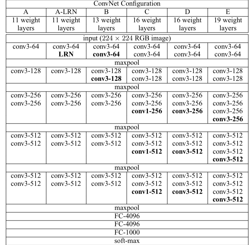
2.2 Configurations

• The ConvNet configurations, evaluated in this paper, are outlined in Table 1.
  Their names(A-E).
  

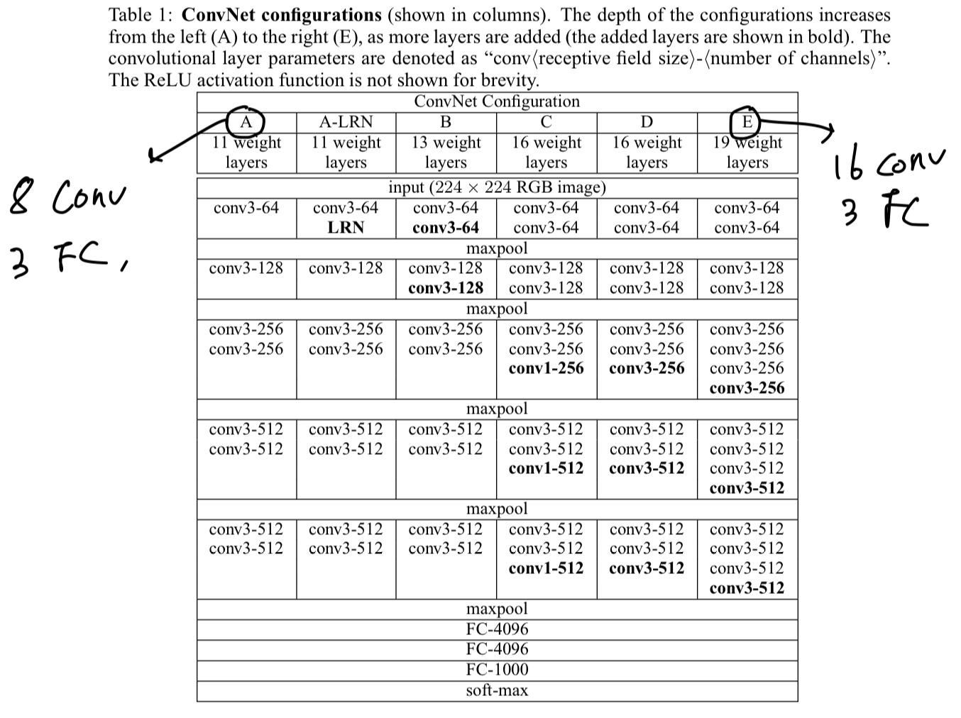
  • All configurations follow in Sect. 2.1 and differ only in the depth(A : 11 layers, E : 19 layers).
  • The width of conv layers(# channels) is starting from 64 in the first layer and then increasing by a factor of 2 after each max-pooling layer, until it reaches 512.

• In Table 2 we report # parameters for each configuration.
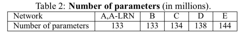  In spite of a large depth, # weights in our nets is not greater than # weights in a more shallow net.

2.3 Discussion

• Our ConvNet configurations are quite different from the ones used in the top-performing entries of the ILSVRC-2012(AlexNet) and ILSVRC-2013 competitions.
  Rather than using large receptive fields in the first con layers, we use very small 3 x 3 receptive fields throughout the whole net.

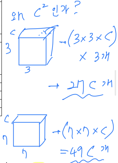
• 우리가 single 7 x 7 layer 대신에 3겹의 3 x 3을 사용해서 얻고자 한 것이 무엇일까?

  1. We incorporate 3 non-linear ReLU layers instead of a single one, which makes the decision function more discriminative.
     (1개 ReLU 쓴 것보다 3번 사용하는게 더욱 잘 decision할 것이다.)
  2. We decrease # parameters.
     만약 3개의 3 x 3 convolution stack이 $C$ 개의 channel을 가졌다고 가정하면, $3(3^2C^2)=27C^2$개의 weights로 되어 있다.
     만약 1개의 7x 7 convolution layer는 $7^2C^2=49C^2$개의 parameter가 필요할 것이다.
     81%의 parameter가 더 필요하다. ($27C + 27C * 0.81 = 48.89C$)
     (내 생각 : 왜 $C^2$인가? 그냥 $27C, 49C$가 맞지 않나?)
     

• The incorporation(포함) of 1 x 1 conv layers is a way to increase the nonlinearity of the decision function without affecting the receptive fields of the con layers.
  Even though in our case the 1 x 1 convolution is essentially a linear projection onto the space of the same dimensionality,
  an additional non-linearity is introduced by the rectification funcion.

---

3. Classification Framework

• In the previous section we presented the details of our network configurations. In this section, we describe the details of classification ConvNet training and evaluation.

3.1 Training

• The ConvNet training procedure generally follows Krizhevsky et al. (2012)
  (except for sampling the input crops from multi-scale training images, as explained later).
  주로 mini-batch gradient descent with momentum을 사용하여 multinomial logistic regression을 수행했다.

  • Batch Size : 256
  • Momentum : 0.9
  • weight decay : 0.0005
  • Dropout regularization ratio : 0.5
  • Learning Rate : initially $10^{-2}$,
    (and then decreased by a factor of 10 when the validations set accuracy stopped improving.)

• The learning was stopped after $370K$ iterations($74$ epochs)
  ➡️ (알 수 있는 점 : 1 epoch에 5K iterations임. 그러면 총 5K개의 mini-batch가 있다는 사실을 알 수 있음.
  총 training data 개수인 1,300,000 / 5,000 = 260 이니까 batch size가 256임을 간접적으로 알 수 있다)

• We conjecture(추론) that in spite of the larger number of parameters and the greater depth of our nets compared to AlexNet, the nets required less epochs to converge due to

  • (a) : implicit regularization imposed by greater depth and smaller conv filter sizes
    ➡️ (나의 생각 : 7 x 7 filter보다 3 x 3 filter를 사용하여 parameter수를 줄였으니 regularization 효과가 생길 수도 있는 것 같아서 맞는 conjecture인 것 같다.)
  • (b) : pre-initialization of certain layers.

• The initialization of the network weights is important.
  We began with training the configuration A(Table 1), shallow enough to be trained with random initialization.
  (Random initialization with the zero mean and $10^{-2}$ variance.)
  그리고 deeper architecture를 학습할 때, we initialized the first four(맨 처음 4개) convolutional layers and the last three FC layers with the layer of net A.
  The biases were initialized with zero.

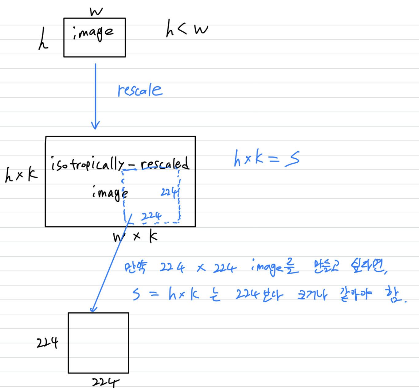
Training image size

• Training image rescaling is explained below.
  Let $S$(= the training scale) be the smallest side of an isotropically-rescaled training image, from which the ConvNet input is cropped.
  (ConvNet input에서 crop된 training image를 rescale한 image에서 길이가 작은 부분을 $S$라고 하자.)
  
  만약 crop size가 224 x 224로 fix되었다면, $S$는 적어도 224보다 크거나 같아야 한다.
  만약 S가 224보다 훨씬 크다면, the crop은 image의 아주 작은 part를 가리킬 것이다.
  (내가 이해한 그림)
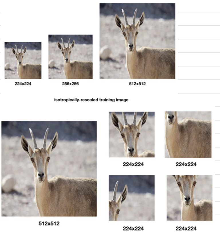  (이해를 돕기 위해 첨부한 사진 : https://ysbstudy.tistory.com/4)

• We consider two approaches for setting the training scale S.

  1. The first is to fix S.
     • Two fixed scale : S=256 and 384.
     • We first trained the network using S=256.
     • To speed-up training of the S=384, it was initialized with the weights pre-trained with S=256.
  2. The second approach to setting S is multi-scale training,
     where each training image is individually rescaled by randomly sampling S from a certain range $[S_{min}=256, S_{max}=512])$.
     • This can also be seen as training set augmentation by scale jittering,
       where a single model is trained to recognizee objects over a wide range of scales.
     • For speed reasons, we trained multi-scale models by fine-tuning all layers of a single-scale model with the same configuration, pre-trained with fixed S=384.

3.2 Testing

• At test time, given a trained ConvNet and an input image,
  it is classified in the following way.
  First it is istropically rescaled to a pre-defined smallest image side, denoted as $Q$(= the test scale).
  We note that $Q$ is not necessarily equal to the training scale $S$
  (test time에서도 또한 isotropically rescaled image를 준비하여, smallest image side를 Q라고 할 것임.
  그리고 Q는 S가 반드시 같을 필요가 없다)
  Then, the network is applied densely over the rescaled test image in a way similar to Sermanet et al., 2014. (https://arxiv.org/pdf/1312.6229.pdf)
  ➡️ 위 paper를 모두 읽어보진 않았지만, 위 model이 the winner of the localization task of the ImageNet Large Scale Visual Recognition Challenge 2013 (ILSVRC2013) 인 것 같다.
  ➡️ VGGNet에 Test image를 넣을 때, multi-scale image를 입력하기 때문에
  고정된 크기의 image를 받아야 하는 fc layer에는 불리하게 작용할 것이다.
  따라서 FC layer를 Conv layer로 대체하여 multi-scale image를 입력하여 prediction할 수 있도록 해주는 기술이 소개된 것 같다.

3.3 Implementation Details

• Our implementation is derived from the publicly available C++ Caffe toolbox.

• But, contains a number of significant modifications,

  • Single system에 multiple GPU가 있어도 training and evaluation을 할 수 있으며, 특히 Full-size(uncropped) images 한 번에 다룰 수 있다.
  • Multi-GPU로의 training은 data parallelism을 기반으로 하여, GPU마다 각 batch의 일부분을 처리할 수 있다.
  • 이렇게 잘려진 batch들의 gradients를 구한 뒤, 평균 내어 full batch의 gradient를 구한다.
  • 이런 방식은 완전한 동기화에 기반하므로, single GPU로 training 하는 것과 동일한 효과를 내면서 더 빠르게 처리할 수 있다.

• Training 소요시간은 NVIDIA Titan Black GPU 4개로 2~3주가 걸렸다.

---

4. Classification Experiments

• Explain about dataset
  • ILSVRC-2012 dataset : they includes images of 1000 classes.
  • Training : 1.3M images
  • Validation : 50K images
  • Testing : 100K images
  • top-1, top-5 error 계산

4.1 Single Scale Evaluation

• The test image size was set as follows:
  Q = S for fixed S,
  and Q = 𝟎.𝟓(𝐒𝐦𝐢𝐧, 𝐒𝐦𝐚𝐱) for jittered S in [𝐒𝐦𝐢𝐧, 𝐒𝐦𝐚𝐱]
  

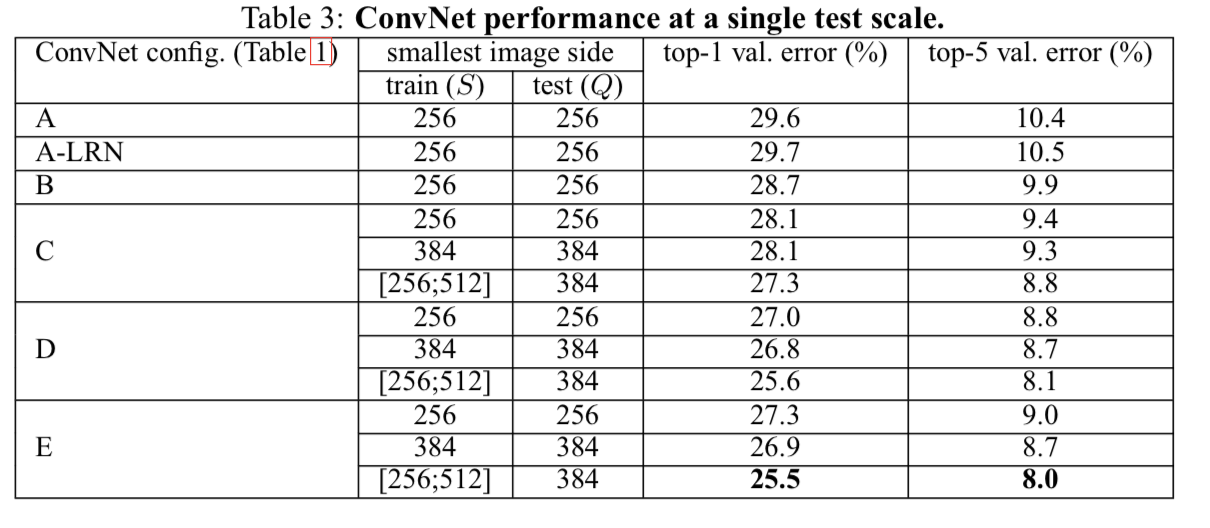
  • A-LRN에서 LRN을 적용했는데 performance 향상에 도움을 주지 않아서 B-E에서는 LRN을 사용하지 않았다
  • same depth임에도 불구하고, 1 x 1 conv layer를 포함한 C는 D보다 안좋은 performance를 보였다.
    ➡️ 이는 Non-linearity를 더하는 것이 도움이 되긴 하지만(C is better than B),
    conv filter를 사용하여 sptial context를 capture하는 것이 더욱 중요해보인다 (D is better than C)

• Training time 동안 scale jittering은 fixed scale을 이용하여 학습하는 것보다 더 나은 결과를 보임.

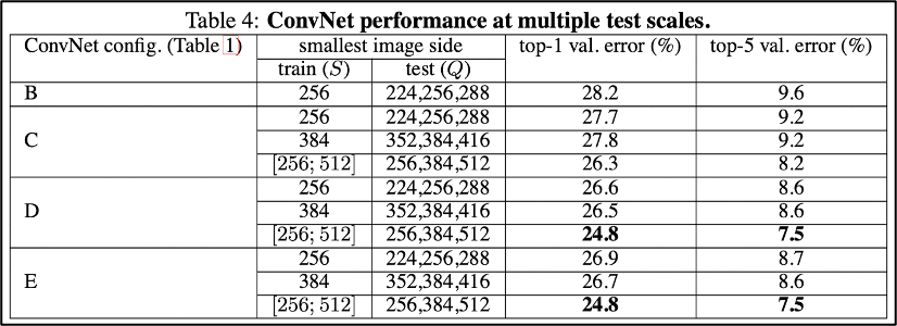
4.2 Multi-Scale Evaluation

• Having evaluated the ConvNet models at a single scale,
  우리는 the effect of scale jittering at test time을 평가하기 위해서
  test할 때에 하나의 Q가 아니라, 3가지의 Q를 사용했다.

  • Training with fixed S, Test : 𝑄={𝑆−32, 𝑆, 𝑆+32}
    training image와 testing image의 크기 차이가 너무 크면 evaluation이 어려울 수 있으니 Q는 +-32로 제한.
  • Training with scale jittering, Test : 𝑄={𝑆𝑚𝑖𝑛, 0.5(𝑆𝑚𝑖𝑛+𝑆𝑚𝑎𝑥 ), 𝑆𝑚𝑎𝑥}
    multi-scale에 대해 학습했으니, 더 다양한 scale에 대해 대응할 수 있을 것이라 생각할 수 있음.

• 결과는 이전과 마찬가지로 depth가 깊은 D, E가 가장 좋았다.
  그리고 scale jittering한 training 결과가 fixed smallest side S로 학습한 것보다 성능이 좋게 나왔다
  

4.3 Multi-Crop Evaluation

• 우리는 multi-crop evaluation과 dense(crop하지 않은 것 같음) ConvNet evaluation을 비교했다.
  
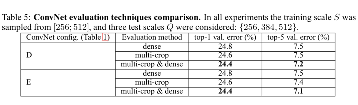
  • using multiple crops performs slightly better than dense evaluation.
  • The two approahces(crop and dense) are indeed complementary.(상호보완적)
    as their combination(multi-crop & dense) outperfoms each of them.

4.4 ConvNet Fusion

• 지금까지는 ConvNet model 각각의 performance를 평가했다.

• 그리고나서
  We combine the outputs of several models by averaging their SoftMax class posteriors.
  (여러 model들의 softmax 이후 값을 averaging함으로써 output을 냈다.)
  ➡️ This improves the performance due to complementarity of the models.

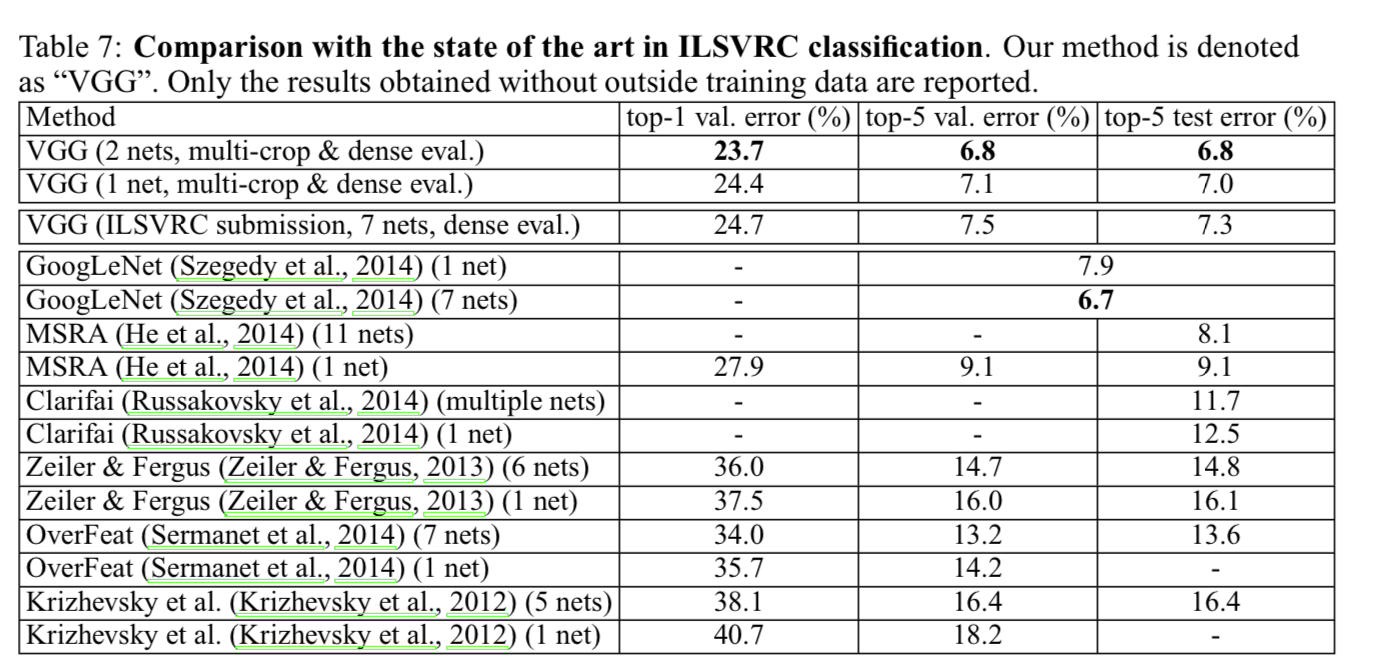
• The resulting Ensemble of 7 networks has 7.3% ILSVRC test error.
  After the submission, we considered an ensemble of only two best-performing multi-scale models(D, E), which reduced the test error to 7.0% using dense evaluation and 6.8% using combined dense and multi-crop evaluation.

4.5 Comparison with the state of the art

• ILSVRC-2014에서 2등을 차지했다.

• 대부분의 ILSVRC 출품작들은 여러 models이 결합된 형태인데, 우리의 ConvNet은 오직 2개의 models만으로 더 좋은 성능을 보였다.

• Notably, we did not depart from the classical ConvNet arch of LeCun et al. (1998),
  but improved it by substantially increasing the depth.

5. Conclusion

• It was demonstrated that the representation depth is beneficial for the classification accuracy, and that state-of-the-art performance on the ImageNet challenge dataset can be achieved using a conventional ConvNet architecture (LeCun et al., 1989; Krizhevsky et al., 2012) with substantially increased depth.

---

Seminar - Discussion

• 대부분의 Parameter들은 FC layer에 있으니까 con layer를 2배로 늘려도 parameter수의 차이가 그렇게 크지 않다.
  그래서 최근의 model은 FC layer가 사라지는 모습을 보인다

• VGGNet은 3개의 3 x 3 conv layer를 사용한 것이다.
  (한 layer에 3 x 3 kernel 3 channels을 사용한 것이 아님)
  ➡️ 1개의 layer보다 3개의 layer는 2개의 ReLU를 더 갖기 때문에 변별력이 더 늘어날 수 있다

• VGGNet의 최대 장점은 단순성이다.
  AlexNet은 언제 overlapping pooling을 써야하는지? 어디 layer에서 Kernel size를 어떻게 해야 하는지? 등의 여러 복잡성이 있는 데에 반해
  VGGNet은 3 x 3 kernel만을 사용하여 단순성을 높였다

• 논문에서 1 x 1 nonlinearity(C)를 증가시키는 것보다 3 x 3 receptive field를 더 살펴보는 것(D)이 중요해 보인다고 했다.
  discussion : 하지만 연산량에 대한 trade-off가 있을 것이다.

• VGGNet은 network 자체는 간단하지만 많은 실험을 했다.
  왜 점수가 잘 나왔는지에 대해 실험을 통해 분석을 해야 한다.
  VGG는 실험적인 논문이라 실험을 많이 보여주지만 다른 논문들은 수학적인 support를 기반한 분석들도 많다.
  하지만 CNN 논문들은 대부분 실험적인 분석이 많다.

• Ablation Study : 의학이나 심리학 연구의 용어이다.
  장기, 조직, 혹은 살아있는 유기체의 어떤 부분을 수술적인 제거 후에 이것이 없을때 해당 유기체의 행동을 관찰하는 것을 통해서 장기, 조직, 혹은 살아있는 유기체의 어떤 부분의 역할이나 기능을 실험해보는 방법을 말한다.
  VGGNet에서도 architecture를 구성하는 하나 하나의 구조들을 뜯어봐서 분석을 했다. (LRN이 있을 때의 결과와 없을 때의 결과, 1 x 1 conv layer가 있을 때의 결과와 없을 때의 결과, ...)
  이렇게 architecture의 구성요소들의 조합을 모두 다 실험을 해봐야 한다.

• GoogleNet을 연구할 때, parameter를 줄이는 것이 목적이었으므로
  144M개의 #parameters를 갖는 VGGNet보다 훨씬 적은 5M개의 #parameters를 갖는다.
  ILSVRC-2012 1위팀 : GooglNet, 2위팀 : VGGNet

• AlexNet에서는 hyper parameter가 너무 많은 옵션이 있었다. (dropout, momentum, LRN에서의 n, 등등...)
  사실 hyper parameter가 많은 것은 좋지 않다. VGGNet처럼 hyperparameter 옵션 없이 고정된 3 x 3 kernel을 사용해서 simple하게 반복적으로 depth를 늘려나가는 것이 더욱 좋다.
  이러한 면에서 CNN 개발에 큰 contribution을 했다고 평가할 수 있다.