Week 2 | Neural Networks Basics | Logistic Regression as a Neural Network
Binary Classification
-
Logistic Regression is an alogirthm for Binary Classification
-
An example of a Binary Classification Problem :
- 어떠한 input image가 있다
그 image에서 cat을 인식할 수 있다면 , 아니면 을 denote하는 output label이 존재

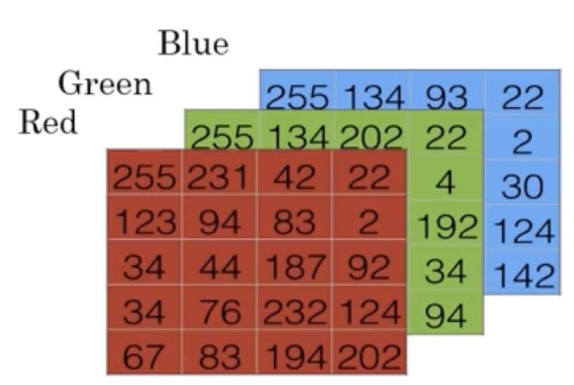
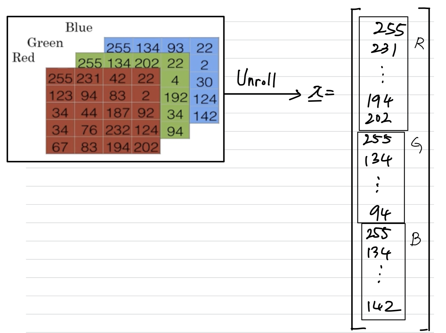
- Computer에서는 위의 image를 어떻게 표현하는지 살펴보자
Computer에서 위의 image를 3가지 Red, Green, Blue color chennels을 matrices로 저장한다.
만약 input image가 X pixel이라면,
image의 RGB pixel intensity values를 일치시키기 위해 X X matrices가 될 것이다.
- X X matrices의 pixel intensity values를
feature vector 로 변환하기 위해서
모든 pixel intensity values를 feature vector로 unroll해야 한다.
feature vector 의 전체 dimension은 X 이 된다. (3 x 64 x 64 = 12,288)
이때, input feature 의 dimension을 로 표현한다.
- 그래서 Binary Classification이란
feature vector 로 나타내는 image를 입력할 수 있는 classifier를 학습하고,
feature vector 에 대응하는 label 가 1인지? 0인지?에 따라
cat image인지? cat image가 아닌지?를 prediction하는 것이 목적이다.
- 어떠한 input image가 있다
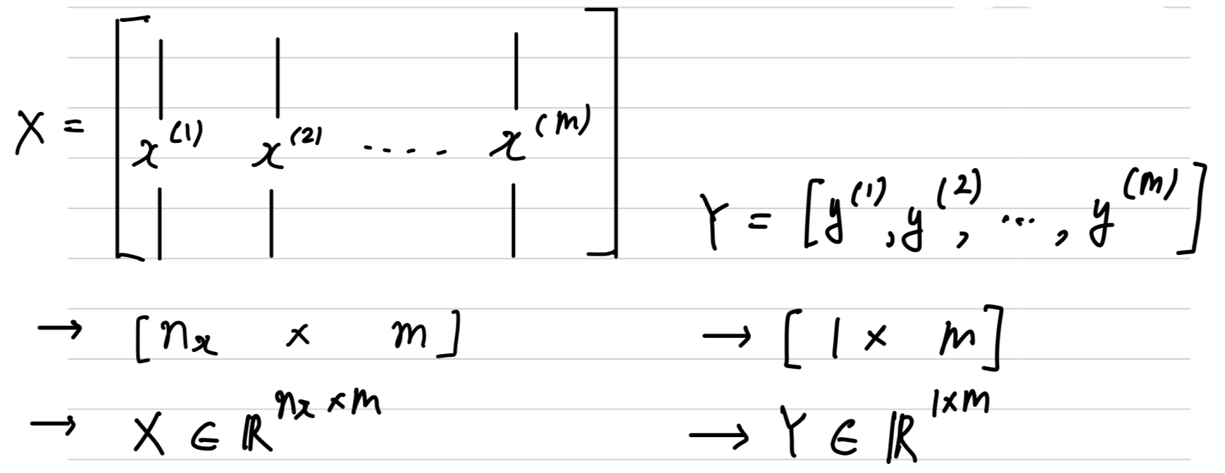
Notation
- pair로 나타내는 single training example :
- {}
- 개의 training examples
first training example: (, )second training example: (, )last training example: (, )training set: { }To emphasize the number of training samples:To output all of the training example: ,
: 한 image의 크기
: 전체 image 개수

Python Command- X.shape = ()
- Y.shape = ()
Logistic Regression
Logistic Regressionis a algorithm that you use when the output labels Y in a supervised learning problem are all either zero or one,
so for binary classification problems.
- input feature vector ():
an image that you want to recognize as either a cat picture or not a cat picture. - Parameters(, )
- Ground Truth label
- estimate of = = :
the chance that this is a cat picture
Notation
How to generalize the output
-
:
This is not a very good algorithm for binary classification.
왜냐하면, 우리는 이 일 확률이 되기를 원한다.
그래서 이 0~1 사이의 값을 갖아야 한다.
하지만 는 1보다 크거나, 음수의 값을 가질 수 있기 때문에
Probability에 합당하지 않다. -
: 따라서 을 sigmoid function, 에 적용한 값을 사용한다.
- (참고) : 다른 교재에서는
= { ,, ..., } ➡️ = {, ..., }, = 으로 다르게 notation하기도 한다.
Sigmoid Function
Sigmoid Functionlooks like
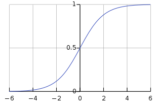
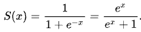
- if is very small,
- if is very large,
Cost Function
-
To train the parameters , of logistic regression model
Wee need to define acost function. -
, where
Given {,..., }, want -
Loss Function = Error Function:
it measures how well you're doing on a single training example.- Squared Error :
➡️ logistic regression에서 보통 사용하지 않는다.
왜냐하면, 나중에 배울 optimization 문제가 non convex하기 때문이다.
if : ➡️ want large, want large (max 1)
if : ➡️ want large, want small (min 0)
- Squared Error :
-
Cost Function:
it measures how are you doing on the entire training set.
Our logistic regression model,
we're going to try to find parameters and
that minimize the overall Cost Function
Gradient Descent
recap:
,
Want to find , that minimize
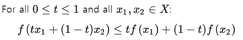
Convex Function
convex function: 간단히 말하면 아래로 볼록한 함수.
이 함수 위의 두 점을 선분으로 이었을 때,
해당 선분 위의 모든 점들이 함수의 점보다 위에 있거나 같은 위치에 있는 함수)
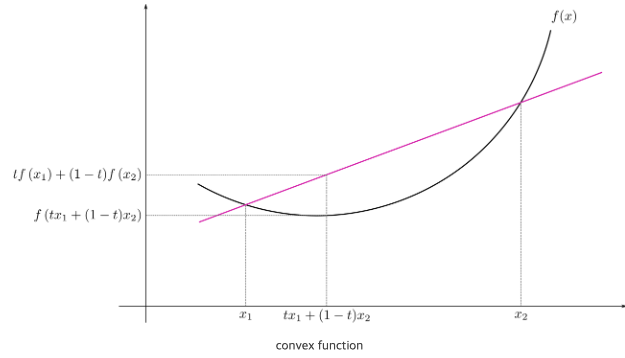
Assumption: Cost Function is a convex function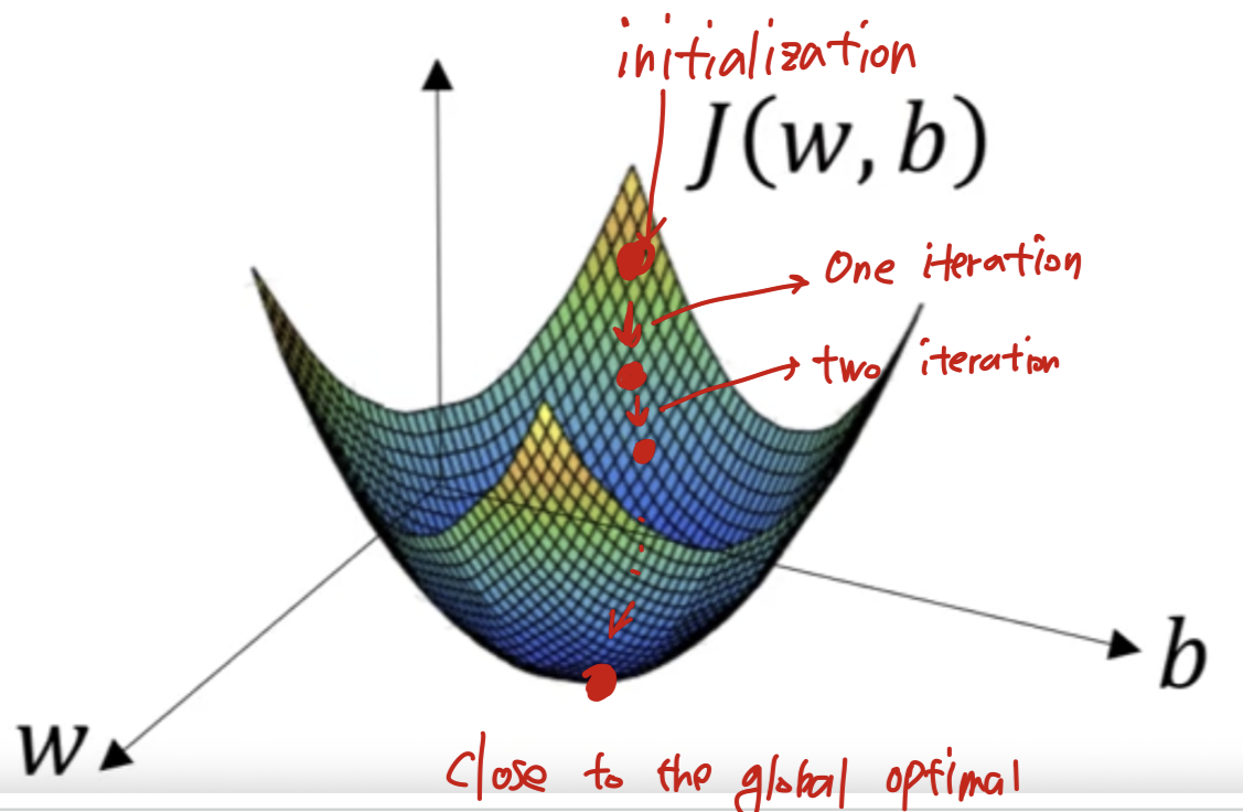
- initialize and :
For logistic regression, almost any initialization method works
보통은 0으로 initialization한다.
Random initialization도 잘 동작하지만,
convex function이라서 어디에 initialization하는지에 관계없이
모두 최저점에 똑같이 도달하기 때문에 보통 사용하지 않는다.
- initialize and :
Gradient descent algorithm: To train or to learn the parameters on our training set.- There's a function that we want to minimize. (그리기 편하기 위해 는 생략)
repeatly carry out the following update
➡️ ( : learning rate)
➡️ ( : learning rate)
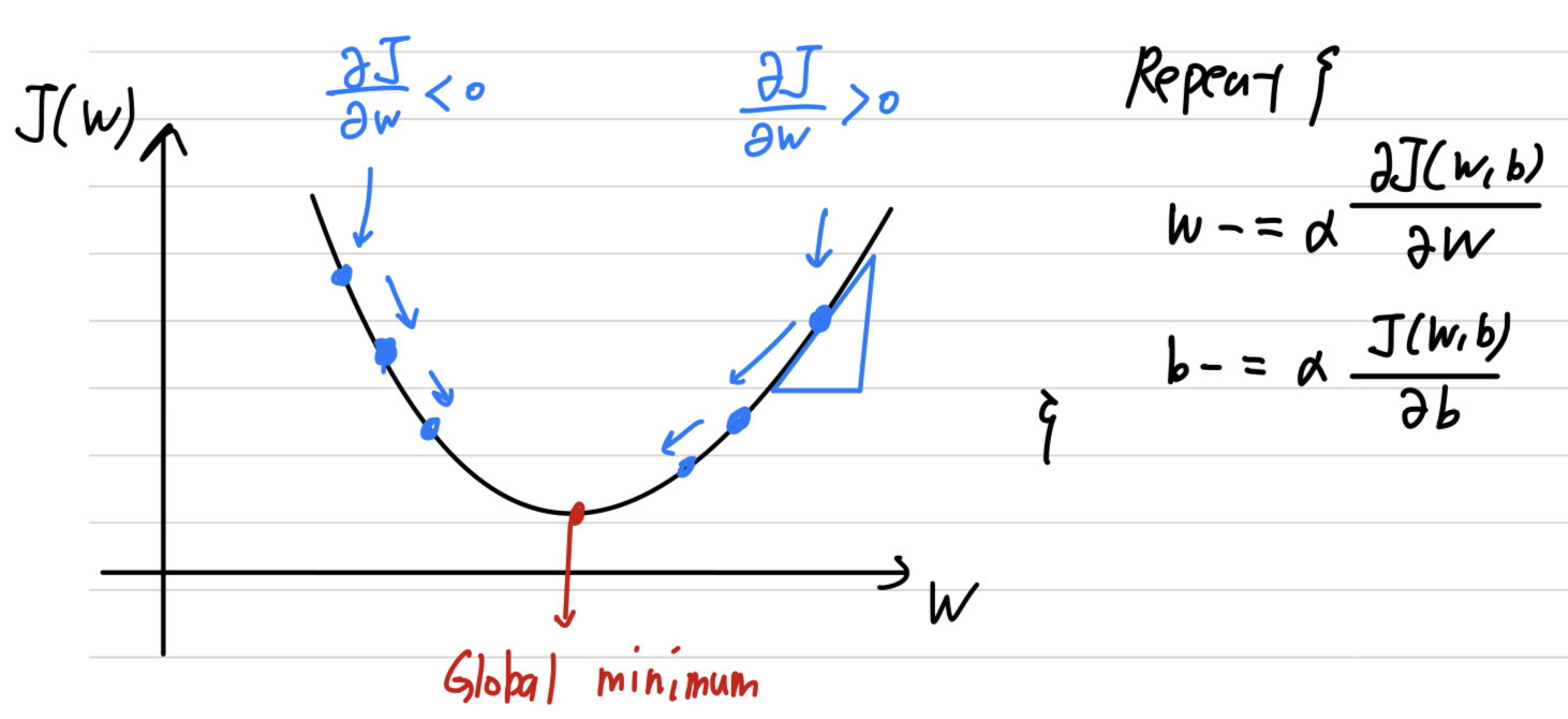
- There's a function that we want to minimize. (그리기 편하기 위해 는 생략)
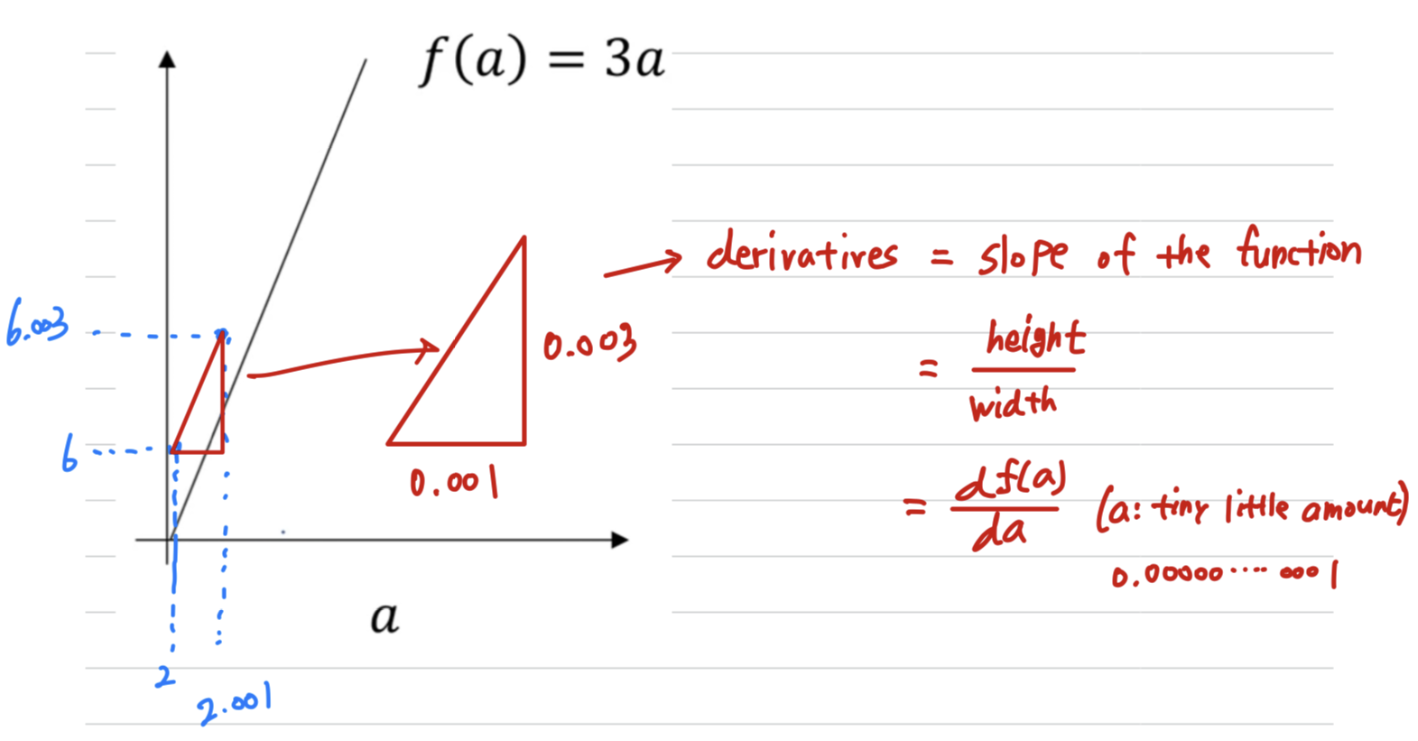
Derivatives
-
Derivative just means slope of a function -
formal definition: This go up three times as much as
whatever was the tiny, tiny, tiny, amount(infinitesimal amount) that we nudged to the right -
아래 예제에서는 직관적인 이해를 위해 0.001 축 방향 0.001 이동시켰지만,
실제 derivatives의 정의는 무한히 작은 값(infinitesimal amount)을 이동시킨다.
Derivatives
= Slop of the function
=
= ( : infinitesimal amount)
More Derivate Examples
- On a straight line, the functions's derivative doesn't change
- The slope of the function can be different points on the curve
formula :
(2와 2.001의 차이 0.001은 infinitesimally small하지 않기 때문에 formula에 의한 값과 오차 존재)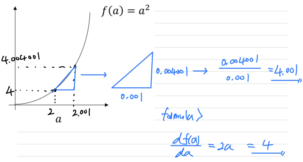
-
formula :- by formula,
we can see that the formula is correct.
➡️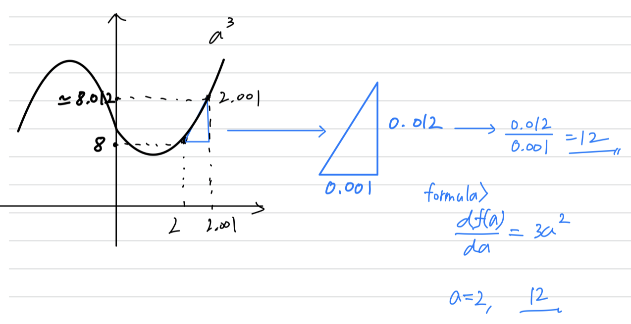
- by formula,
-
formula :- by formula,
we can see that the formula is correct.
➡️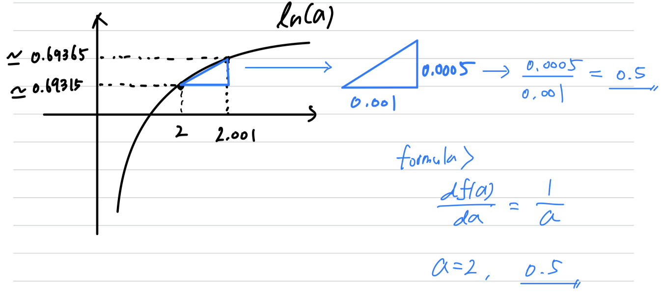
- by formula,
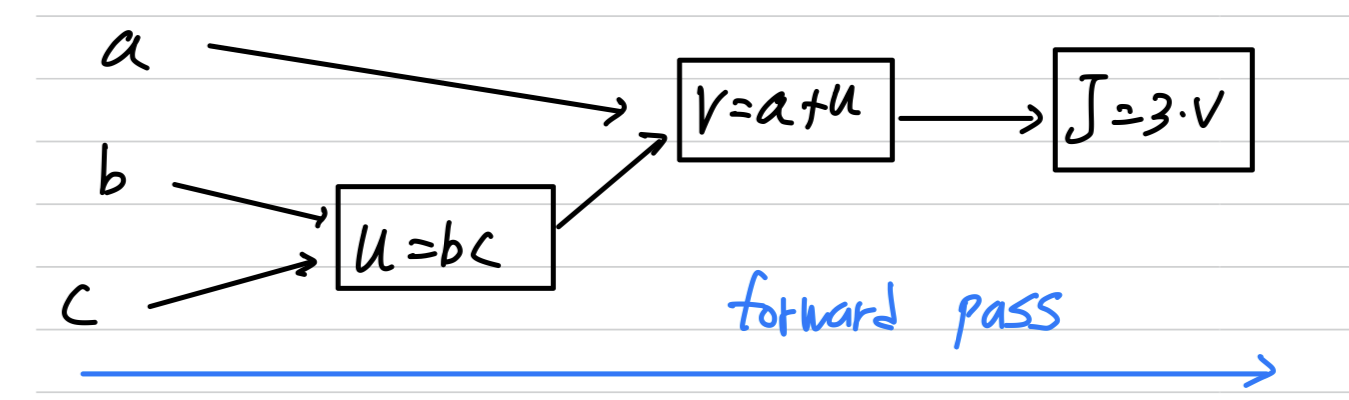
Computation Graph
-
The computation of a neural network are organized in terms of a
forward pass(= forward propagation step) in which we compute the output of the neural network
followed by abackward pass(= backward propagation step) which we use to compute gradients or compute derivatives. -
The computation graph explains why it is organized this way
-
Simple example:
변수 를 사용하는 function 가 있다고 가정하자.- 는 총 3단계로 나눌 수 있다.
Derivatives with a Computation Graph
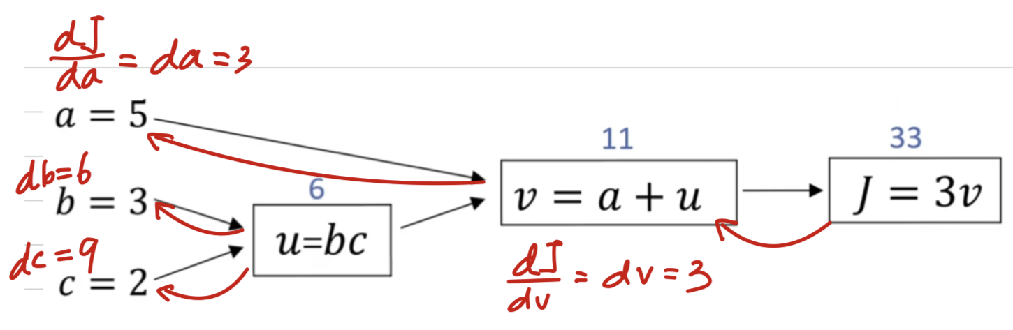
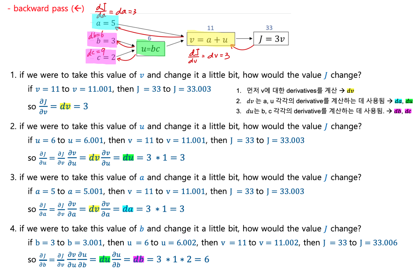
Key Point:
Computing all of these derivatives,
the most efficient way to do so is through a right to left computation
following the direction of the red arrows.
1. 먼저 에 대한 derivatives를 계산
2. 그러면 에 대한 derivative와 에 대한 derivative를 계산하는 데 유용.
3. 그러면 , 각각에 대한 derivative 계산하는 데 유용
Logistic Regression Gradient Descent
- 하나의 training example에 대해서
Logistic Regression에 대한 Gradient Descent를 수행하는 방법을 살펴보자.
- : output of logistic regression
- : ground truth label
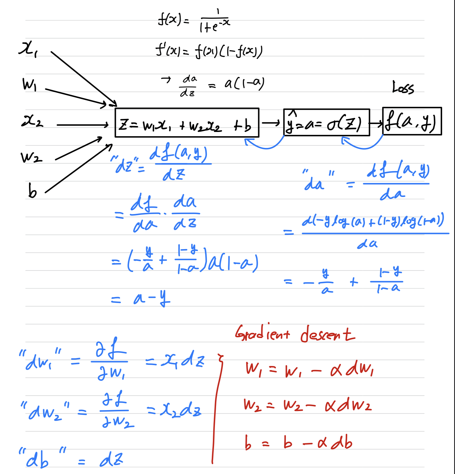
Gradient dsecent on m examples
remind:
- 앞서 하나의 training example()만 갖고 계산했던 derivatives :
Logistic regression on m examples:
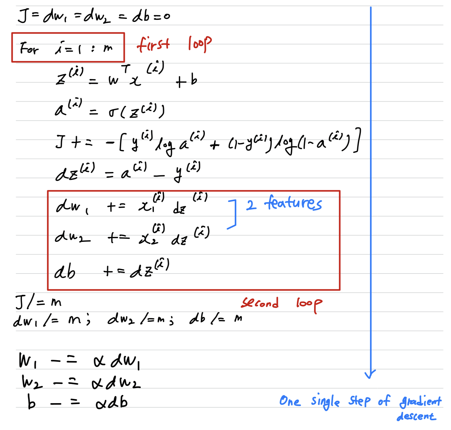
- But, we need to write two for loops
- first for loop : 개의 training example에 대한 for loop
- second for loop : for loop over all the features()
만약 feature가 개가 된다면, feature 개에 대한 for loop이 필요.
- 만약 deep learning algorithm을 구현할 때, for loop이 있으면 algorithm 효율이 떨어진다.
deep learning 시대에는 dataset이 매우 커지기 때문에
명시적 for loop를 사용하지 않고 algorithm을 구현할 수 있어야 한다.
그러기 위해서vectorization이 매우 중요해졌다.
- But, we need to write two for loops
