paper info

• paper : Pruning Filters for Efficient ConvNets
• Published as a conference paper at ICLR 2017
• authors : Hao Li, Asim Kadav, Igor Durdanovic, Hanan Samet, Hans Peter Graf

---

0. Abstract

• CNNs이 다양한 application에 성공을 거두는 것은 computation과 parameter stroage cost를 상당히 증가시키고 있어서,
  최근 original accuracy 손해 없이 layer들의 weight들을 purning하고 compressing하여 이러한 overhead를(computation과 parameter stroage cost 증가) 줄이는 연구가 활발히 진행되고 있다.

• (이전의 deep compression 방법의 문제점 지적) :
  하지만 weight의 magnitude-based pruning은 fully connected layer의 많은 중요한 parameter를 없애고,
  pruned network의 irregular sparsity로 인해 convolutional layer에서는
  computation cost를 부적절하게 줄이게 될 것이다.

• (새롭게 제안하는 방법) :
  우리는 CNN의 output accuracy에 작은 영향만 미친다고 확인된
  acceleration method인 prune filter를 소개할 것이다.

• feature map과 연결된 모든 filter들을 제거함으로써, computation cost는 매우 감소된다.
  pruning weight에 반하여, 이러한 방법은 sparse connectivity pattern을 만들지 않는다.
  이러한 이유로, 우리가 제안한 아이디어는 sparse convolution libraries(cuSPARSE)의 도움이 필요 없고,
  dense matrix multiplication을 위한 BLAS library에 효율적으로 작동할 수 있다.

• 우리는 훨씬 간단한 filter pruning technique으로 CIFAR 10에 대해서
  network를 retraining함으로써 original accuracy에 가깝도록하여
  VGG-16을 34%, ResNet-110을 38%의 inference cost를 줄일 수 있었다.

---

1. Introduction

• ImageNet challenge는 CNNs architectural choices에 많은 발전을 이루게 했다.
  
  최근 trend는 network의 parameter와 convolution operation을 늘리며 deeper하게 만드는 것이다.
  이러한 high capacity network는 특히 embedded sensor나 mobile device처럼
  computational and power resource가 제한되어 있는 것들과 함께 사용되기에
  매우 큰 inference cost가 필요하다.

• 그래서 최근 model compression으로 storage and computation costs를 줄이는 연구들이 많이 진행되고 있다.
  
  그 중에서 최근 Learning both Weights and Connections for Efficient Neural Network.(Song Han, Jeff Pool, John Tran, and William Dally. In NIPS, 2015.)에서는
  AlexNet과 VGGNet에 대해
  pruning weights with small magnitudes and then retraining without hurting the overall accuracy를 함으로써 인상적인 compression rates를 보여줬다.
  

• 하지만
  fully connected layer에서 제거된 parameter들의 computation cost는 낮기 때문에
  parameter를 pruning하는 것은 반드시 computation cost을 줄이지 않는다.
  예를 들어, VGG-16의 fully connected layer의 parameter가
  total parameter 개수 중의 90%를 차지하지만,
  전체 floating point operations(FLOP)에는 1% 미만 밖에 되지 않는다.
  
  이 논문에서는 또한 convolutional layer가 compressed되고 accelerated될 수 있다고 증명했지만,
  추가적으로 sparseBLAS libraries or specialized HW가 필요하다.
  CNN에 대한 sparse operation을 사용하는 최근의(2016년) library들은 종종 제한적이며(https://arxiv.org/abs/1409.4842),
  sparse data structure를 유지하는 것은 또한 additional storage ovehead를 발생킨다.

• 최근 CNNs에 대한 연구는 다양한 efficient deep architecture를 산출하고 있다.
  그 중에 FC layer를 Average pooling layer로 바꾸는 것도 있었고 그것은 parameter수를 많이 줄일 수 있다.
  computation cost 또한 feature maps의 size를 미리 줄이기 위해 image를 downsampling하는 방식도 있었다.
  하지만 그럼에도 불구하고,
  network가 계속해서 deeper해질수록,
  covnolutional layer의 computation cost는 계속해서 증가할 수 밖에 없다.

• large capacity를 갖는 CNNs은 보통 filter와 feature channel 사이에 많은 redundancy(중복)을 갖고 있다고 알려져 있다.
  이 연구에서, 우리는 well-trained CNNs에 filter를 pruning함으로써 computation cost를 줄이는 것에 집중했다.
  
  weight를 pruning하는 것과 비교하여, filter pruning은
  sparsity를 만날 필요 없이 자연스럽게 구조화된 pruning 방법이므로
  sparse libraries들을 사용하거나 any specialized HW를 사용할 필요가 없다.
  
  pruned filte는 matrix mlutiplization 숫자를 줄임으로써 직접적으로 acceleration과 관련되어있다.
  추가적으로, layer-wise iterative fine-tuning 대신에,
  우리는 많은 layer들에 대해 filter를 pruning하는 retraining time을 절약하기 위해서
  one-shot pruning과 retraining strategy를 적용했다.
  그리고 one-shot pruning은 very deep network에 매우 중요하다.

• 마침내 우리는 AlexNet or VGGNET보다 특히 ResNet에서
  상당히 적은 parameter와 inference cost를 갖는다고 관찰했다.
  (아주 약간의 accuracy 손해를 봤지만 30%의 FLOP reduction)
  우리는 ResNet을 더 잘 이해하기 위해 ResNet의 convolutional layer에 대한 sensitivity analysis를 수행했다.

---

2. Related Work

• 과거의 weight pruning 연구 :
  과거 Optimal Brain Damage, Le Cun et al. (1989)에서는 이론적으로 정의된 saliency measure(특징이되는 값)을 이용해서 weight를 prune했다.
  나중에, Second Order Derivatives for Network Pruning: Optimal Brain Surgeon, Hassibi & Stork (1993)에서는 second-order derivative information에 의해 결정된 unimportant weight들을 제거하는 Optimal Brain Surgeon을 제안했다.
  하지만, 이러한 방법들은 단지 fully-connected layer에서만 동작하고, sparse connections이 발생한다.

• 과거의 computation cost 줄이는 연구 :
  과거의 연구에서는
  convolutional layer의 computation cost를 줄이기 위해서,
  원래의 filter 개수를 바꾸지 않고
  두개의 작은 matrices들의 low rank product로 weight matrix를 나타냄으로써 convolutional operation을 approximate하는 것을 제안했다.
  (Denil et al. (2013); Jaderberg et al. (2014); Zhang et al. (2015b;a); Tai et al. (2016); Ioannou et al. (2016))
  
  convolutional overheads를 줄이기 위한 다른 approach들은
  FFT based convolutions, fast convolution using the Winograd algorithm 을 포함한다.
  추가적으로 quantization과 binarization도 model size를 줄이고 computation overhead를 줄이는 데에 사용될 수 있다.

• 과거의 redundant를 줄이는 연구 :
  well trained network로 부터 중복되는 feature map들을 제거하는 연구들도 진행되어 왔다.
  Anwar et al.(2015)에서는
  3-level pruning of the weights와
  random으로 생성된 mask들 중에서 best combination을 선택하는 particle filtering을 사용하여 pruning candidate들을 찾아냈다.
  Polyak&Wolf(2015)에서는
  face detection applications을 위한 sample input data로 자주 등장하지 않는 activated feature map을 detect했다.
  ➡️ 우리는 가능한 조합들을 검사해볼 필요 없이,
  a simple magnitude based measure를 이용하여
  filter weight와 prune filter가 feature map과 일치하는지에 대한 분석을 통해 고를 것이다.

• 동시에,
  우리의 연구는 sparse constraints(Lebedev & Lempitsky (2016); Zhou et al. (2016); Wen et al. (2016))를 compact CNNS을 훈련시키는 것에 대한 관심이 증가하고 있습니다.
  Lebedev & Lempitsky (2016)에서는 structured brain damage를 이루기 위해
  convolution group filter에 대한 group-sparsity를 사용했다.
  Zhou et al. (2016)에서는 제거된 filter로 compact해진 CNNs을 훈련시기키 위해 training 동안에 group-sparse regularization을 추가했다.
  Wen et al. (2016)에서는 각 layer에 필요없는 filters, channel 또는 심지어 layer들을 없애기 위해서
  각 layer에 structured sparsity regularizer를 추가했다.
  filter-level pruning에서, 위 모든 연구는 $l_{2,1}$norm을 regularizer로 사용한다.
  
  
  위 연구들과 비슷하게 우리는 unimportant filter를 선택하기 위해 $l_1$-norm을 사용했고,
  unimportant filter들을 물질적으로 prune하였다.
  우리의 fine-tuning process는 추가적인 regularization을 제외하면,
  conventional training procedure과 같다.
  우리의 방식은 stage-wise pruning을 적용함으로써,
  한 stage에 모든 layer들에 대한 a single pruning rate를 설정할 수 있다.

---

3. Pruning Filters and Feature Maps

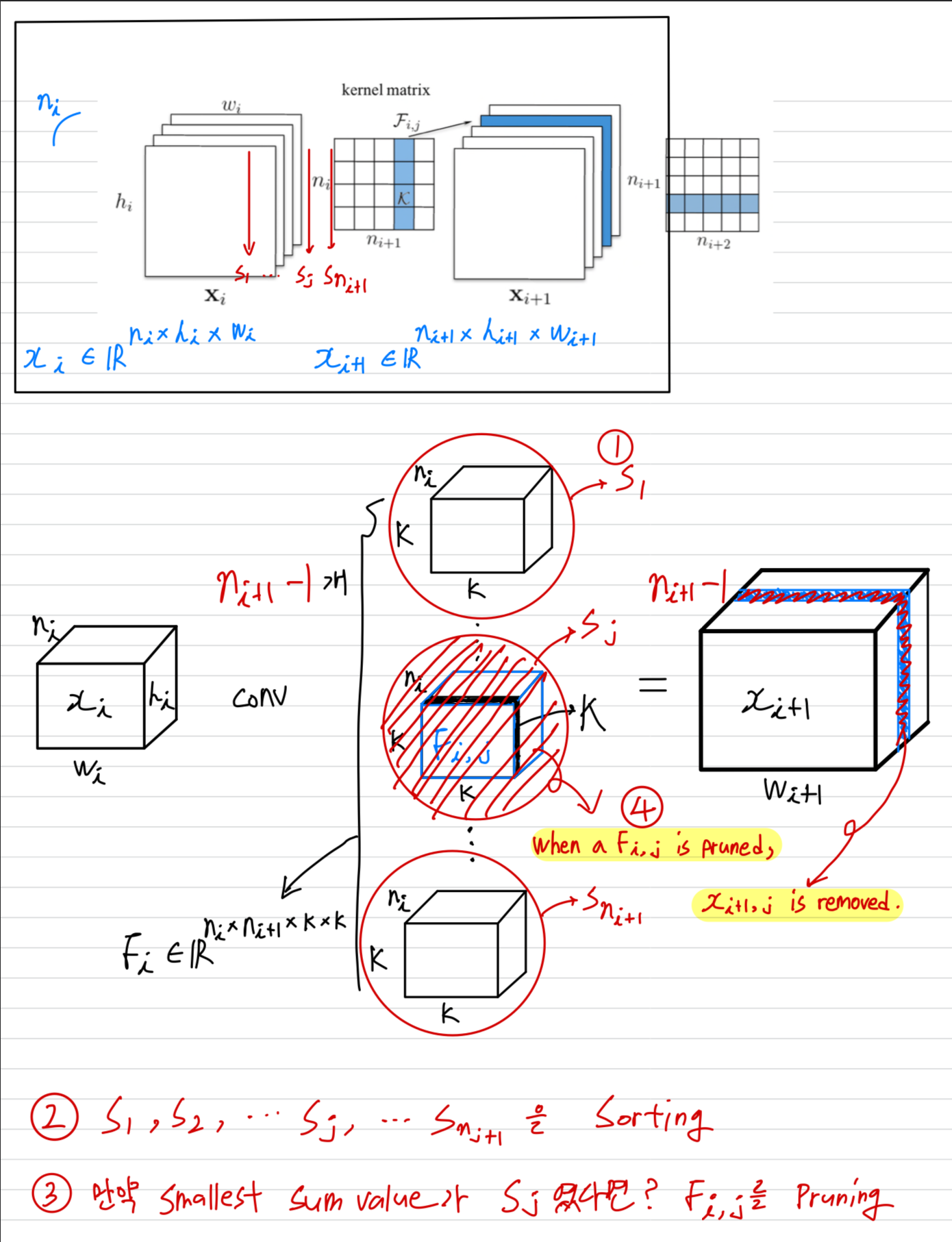
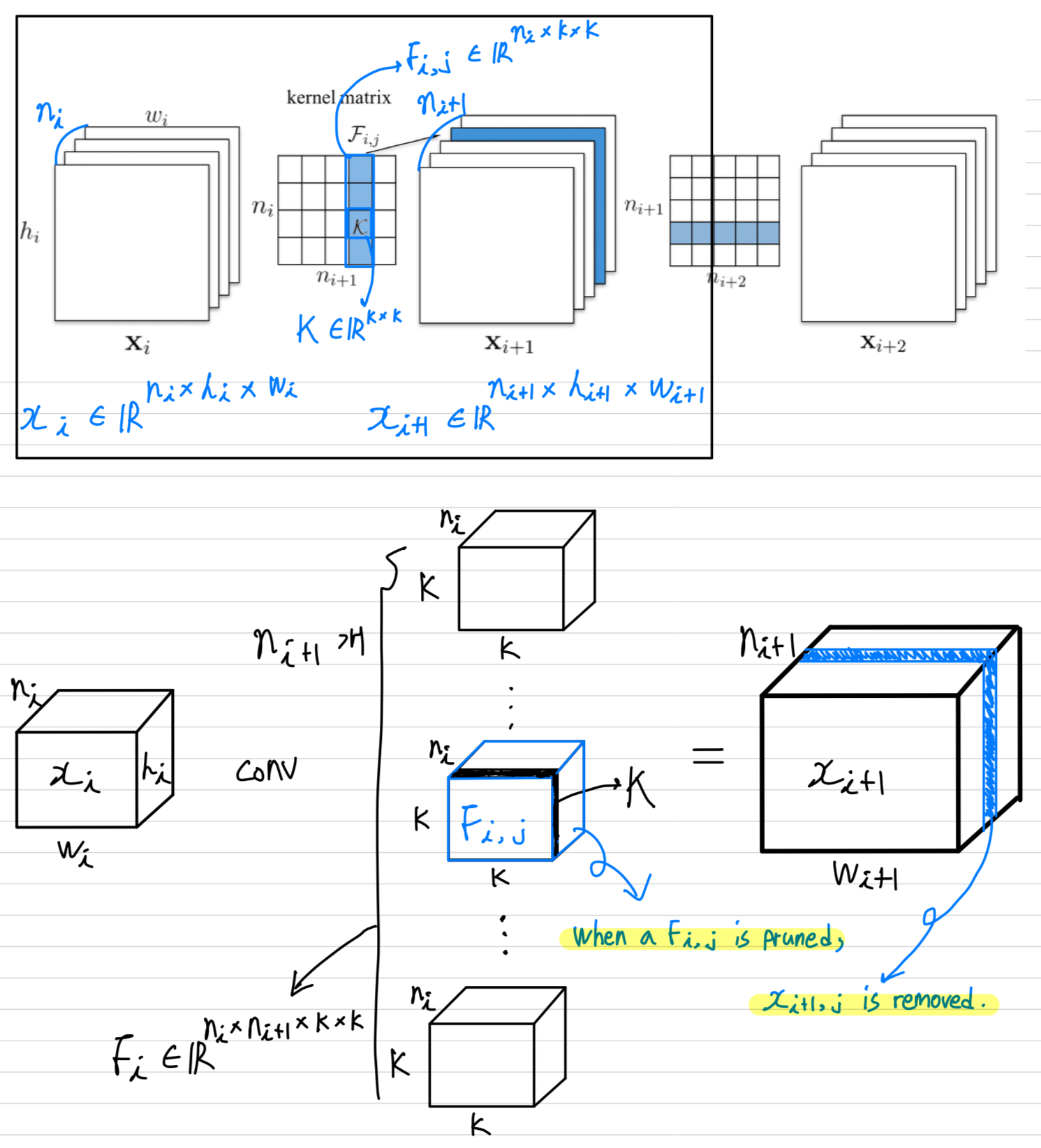
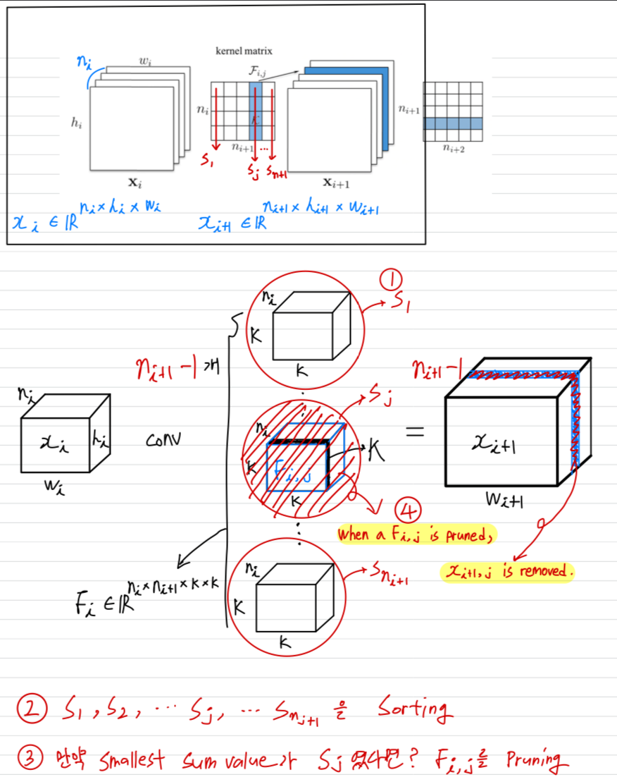
• Let $n_i$ denote the number of input channels for the $i$th convolutional layer and $h_i$/$w_i$ be the height/width of the input feature maps.
  The convolutional layer transforms
  the input feature maps $x_i \in R^{n_i * h_i * w_i}$
  into the output featrue maps $x_{i+1} \in R^{n_{i+1} * h_{i+1} * w_{i+1}}$
  This is achieved by applying $n_{i+1}$ 3D filters $F_{i, j} \in R^{n_i * k* k}$ on the $n_i$ input channels,
  in which one filter generates one feature map.
  Each filter is composed by $n_i$ 2D kernel $K \in R^{k * k}$.
  
  All the filters, together, constitue the kernel matrix $F_i \in R^{n_i * n_{i+1} * k * k}$.
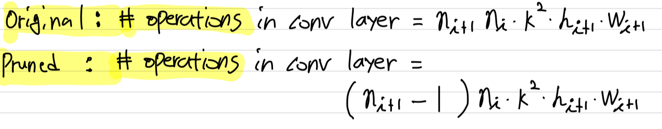
  The number of operations of the convolutional layer is $n_{i+1}n_{i}k^2h_{i+1}w_{i+1}$.
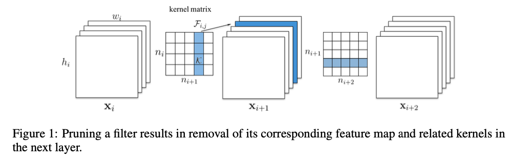
  As shown in Figure 1, when a filter $F_{i, j}$ is pruned,
  its corresponding feature map $x_{i+1, j}$ is removed, which reduces $n_{i}k^2h_{i+1}w_{i+1}$ operations.
  The kernels that apply on the removed feature maps from the filters of the next conv layer are also removed,
  which saves an additional $n_{i+2}k^2h_{i+2}w_{i+2}$ operations.
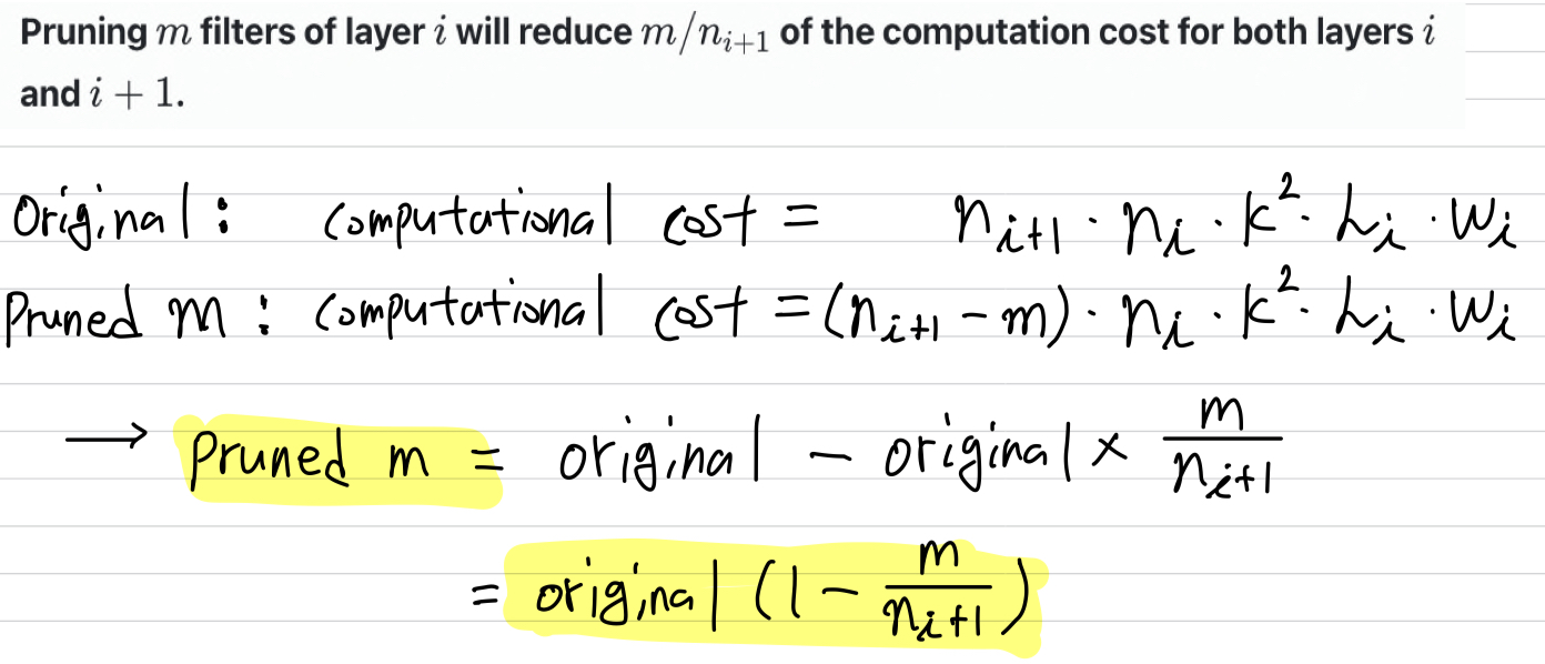
  Pruning $m$ filters of layer $i$ will reduce $m/n_{i+1}$ of the computation cost for both layers $i$ and $i+1$.
  

3.1 Determining which filters to prune within a signle layer

• 우리의 방법은 accuracy drop을 최소화하면서 computational efficiency를 위해,
  well-trained model로부터 less useful filters를 pruning한다.
  우리는 예를 들어, $||F_{i,j}||_1$처럼 $l_1$-norm을 이용하여 $\Sigma|F_{i,j}|$의 weight들의 절대값의 합을 계산함으로써,
  각 layer의 relative importance(상대적 중요도) of a filter를 측정한다.
  $l_1$-norm 예시 : $F_{i,j} = [1, -3, 5]$ ➡️ $\Sigma|F_{i,j}|$ = |1 + 3 + 5| = 9
  
  input channel 개수인 $n_i$는 filter 간에 동일하기 때문에
  $||F_{i,j}||_1$는 또한 kernel weights의 average magnitude를 나타낼 것이다.
  즉, $||F_{i,j}||_1$ value는 output feature map의 크기에 대한 expectation을 줄 것이다.
  Filters with smaller kernel weights는 같은 layer의 다른 filter들과 비교했을 때,
  약한 activation을 갖는 feature maps을 만드는 경향이 있다.
  
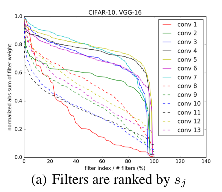
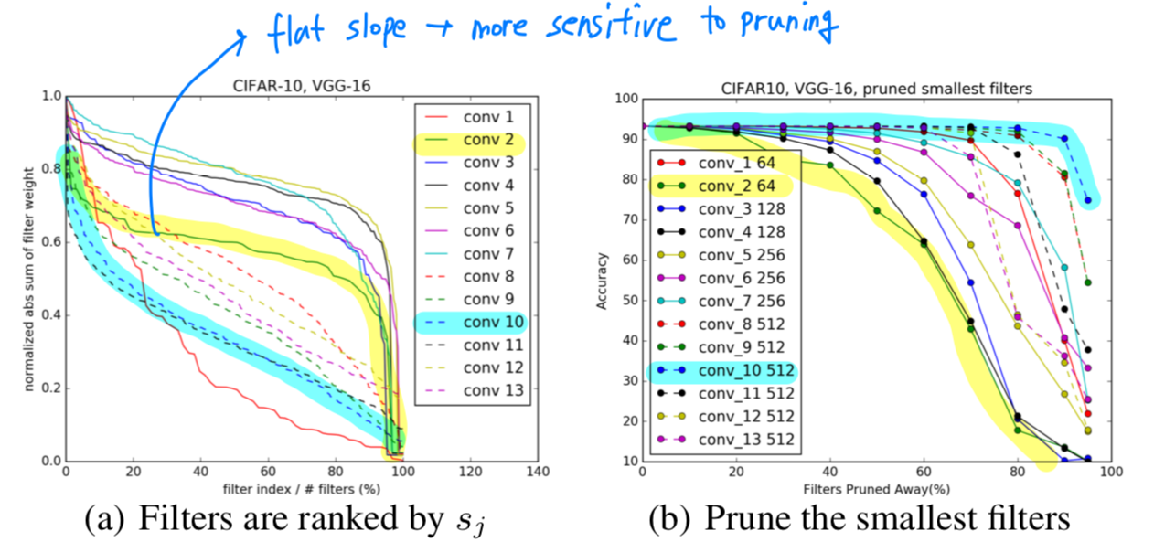
  Figure 2(a)에서는 CIFAR-10 dataset에 훈련된 VGG-16 network의 각각의 convolutional layer에 대한 filter's absolute weights sum의 distribution을 나타내고 있다.
  여기서 distribution은 layer마다 크게 다르다.
  우리는 Section 4.4에서
  random 또는 largest filters에 대해 똑같은 개수로 pruning을 한 것과 비교했을 때,
  smallest filters를 pruning하는 것이 더욱 효과적인 것을 알아냈다.
  
  또한 우리는 Section 4.5에서
  activation-based feature map pruning에 대한 다른 기준들과 비교했을 때,
  $l_1$-norm이 data-free filter selection에 대한 좋은 기준이라고 알아냈다.

• $i$번째 convolutional layer로부터 $m$개의 filters를 pruning하는 과정은 다음과 같다.
  1. 각 filter $F_{i,j}$에 대해서,
     the sum of its absolute kernel weights $s_j=\Sigma_{l=1}^{n_i}|K_l|$을 계산한다.
  2. $s_j$에 의해 filters들을 정렬한다.
  3. smallest sum values 와 그에 해당하는 feature maps $m$개를 pruning한다.
  4. $i$th와 $i+1$th layer 사이의 새로운 kernel matrix가 생성되었고,
     나머지 kernel weights들은 새로운 model로 copy되어진다.
     

Relationship to pruning weights

• Magnitude-based pruning에서
  모든 filter의 kernel weight들이 threshold보다 작을 때,
  전체의 filter가 pruning되어질 수 있다.
  하지만따라서 threshold의 신중한 tuning이 필요하고,
  최종적으로 제거될 filter의 정확한 개수를 예상하는 것이 어렵다.

Relationship to group-sparse regularization on filters

• 최근 연구 Less Is More: Towards Compact CNNs, Zhou et al. (2016)에서
  convolutional filter에 group-sparse regularization($\Sigma_{j=1}^{n_i}||F_{i,j}||_2$)을 적용했고,
  그것은 또한 작은 $l_2$-norm을 갖는 filter들을 zero-out하였습니다.
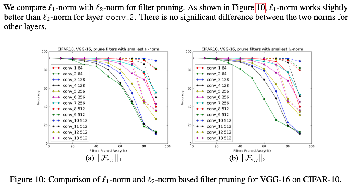
  하지만 실제로, 우리는 filter selection을 위한 $l_2$-norm과 $l_1$-norm의 차이를 눈에 띌만하게 관찰하지 못했다. (Appendix 6.1)
  training 동안에 많은 filter들의 weight들을 zeroing out하는 것은
  Section 3.4에서 소개하는 iterative pruning and retraining 전략으로 filter를 pruning하는 것과 비슷한 효과가 있다.

3.2 Determining single layer's sensitivity to pruning

• 각 layer에 대한 pruning의 sensitivity를 이해하기 위해,
  우리는 각 layer를 독립적으로 prune한 뒤,
  validation set에 대한 pruned network의 accuracy를 관찰하였다.

• Figure 2(a)에서 larger slope를 갖는 layer에 대응하여
  Figure 2(b)에서 accuracy를 유지하는 것을 관찰할 수 있습니다.
  반면에, 상대적으로 flat slope를 갖는 layer들은 pruning에 더욱 sensitive합니다.
  ➡️ abs sum of filter weight의 값이 골고루 분포되어 있는 경우 = flat slope = more sensitive to pruning
  ➡️ abs sum of filter weight의 값이 골고루 분포되어 있지 않고, 중앙에 몰려있는 값이 많은데 가끔 매우 크고 작은 값을 보이는 경우 = larger slope = less sensitive to pruning
  우리는 pruning에 대한 각 layer들의 sensitivity를 기반하여 경험적으로
  각 layer에 prune할 filter의 개수를 결정했다.
  VGG-16과 ResNet과 같은 deep network에서,
  우리는 같은 feature map size를 갖는 stage의 layer는 pruning에 대한 비슷한 sensitivity를 갖는 것을 관찰했다.
  pruning에 sensitive한 layer들에 대해서,
  우리는 매우 작은 percentage를 pruning하거나 아예 pruning하지 않고 넘겼다.

3.3 Pruning filters across multiple layers

• 이제부터 network 전체에서 filter를 pruning하는 방법을 discussion해보자.
  이전에 연구에서 layer별로 weight를 iteratively retraining 하였고,
  accuracy의 loss에 대해서 보상해줬다.

• 하지만 multiple layer에 대해 어떤 filter를 pruning할건지 한 번에 알아내는 것은 매우 유용하다.

  1. deep network에서는,
     layer 마다마다 pruning and retraining하는 것인 매우 time-consuming하다.

  2. network 전체의 layer를 pruning하는 것은
     network의 robustness를 전체적인 관점에서 파악할 수 있어 network 규모를 작게 만들 수 있다.
     따라서 complex network에서는, holistic approach(전체적인 접근)가 필수적일지 모른다.
     예를 들어 ResNet의 경우,
     identity feature map을 pruning하거나 각 residual block의 두번째 layer를 pruning하는 것은
     다른 layer의 추가적인 pruning을 초래한다.
     

     내 생각 :
     따라서 layer마다마다를 보는 것이 아니라 전체 network를 알아야 network를 위한 Pruning을 더 잘 할 수 있을 것이다.

• multiple layer에 대한 filter를 pruning하기 위해
  우리는 layer-wise filter selection에 대한 2가지 strategies를 고려한다.

  1. Independent pruning은
     각 layer에서 어떤 filter가 pruned되어질지는 다른 layer들에 독립적으로 결정되어야 한다.
  2. Greedy pruning은 previous layer에서 제거된 filter들에 대해서 설명한다.
     이 방법은 the sum of absolute weights가 계산되는 동안에
     이전에 pruned되어진 feature map에 대한 kernel을 고려하지 않는다.

• Figure 3에서는 the sum of absolute weights에 대한 두 접근법의 차이점을 설명하고 있다.
  greedy approach는 globally optimal이 아니더라도,
  특히 많은 filter들이 pruned될 때 higher accuracy를 갖는 pruned network를 만든다.
  

  • The independent pruning strategy는
    previous layer에서 제거되어진 channel을 포함하여
    filter sum을 계산한다.
    그래서 노란색으로 mark되어진 kernel weight가 계속해서 포함되고 있는 것이다.

  • The greedy pruning strategy는 이미 제거된 channel은 고려하지 않고 filter sum을 계산한다.
    
    두 방식은 filter sum($l_1$-norm)을 계산하는 방식일 뿐,
    두 방식 모두 여전히 parameter는 $(n_{i+1}-1)$ x $(n_{i+2}-1)$ kernel matrix를 갖는다.

    정리
    1) independent pruning 방식은 pruned되어진 feature map이 존재하지만,
    다음 layer의 input에 pruned feature map을 사용하지 않고 pruned되지 않은 원래의 feature map을 사용한다.
    다음 layer의 input에만 pruned되지 않은 원래의 feature map을 사용하는 것이기 때문에
    최종적으로는 $(n_{i+1}-1)$ x $(n_{i+2}-1)$ kernel matrix를 갖는다.
    다음 layer에서
    2) greedy pruning 방식은 pruned되어진 feature map이 존재하고,
    그 feature map을 다음 layer의 input으로 그대로 사용하는 것이다.
    마찬가지로 최종적으로 $(n_{i+1}-1)$ x $(n_{i+2}-1)$ kernel matrix를 갖는다.

• VGGNet과 AlexNet같이 simpler CNNs에 대해서,
  우리는 아무런 convolutional layer에서 아무런 filter를 prune할 수 있었다.
  하지만, Residual networks와 같은 complex network에 대해서, pruning filters는 직관적이지 않다.
  ResNet architecture는 pruning하는 것에 restriction이 있고, 신중함을 요구한다.
  
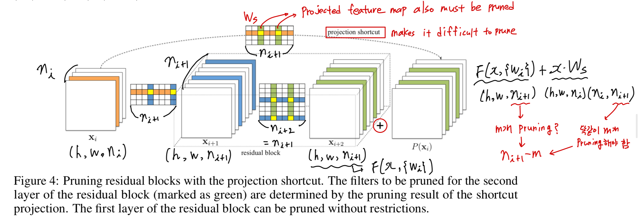
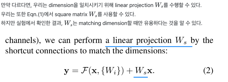
  Figure 4.에서 projection mapping을 갖는 residual block에 대한 filter pruning을 보여준다.
  (우선 projection mappping에 대한 간단한 recap)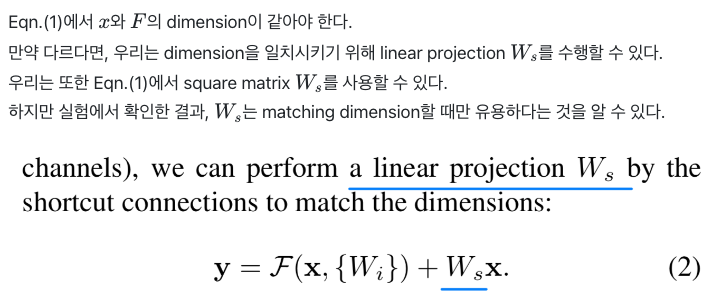여기서,
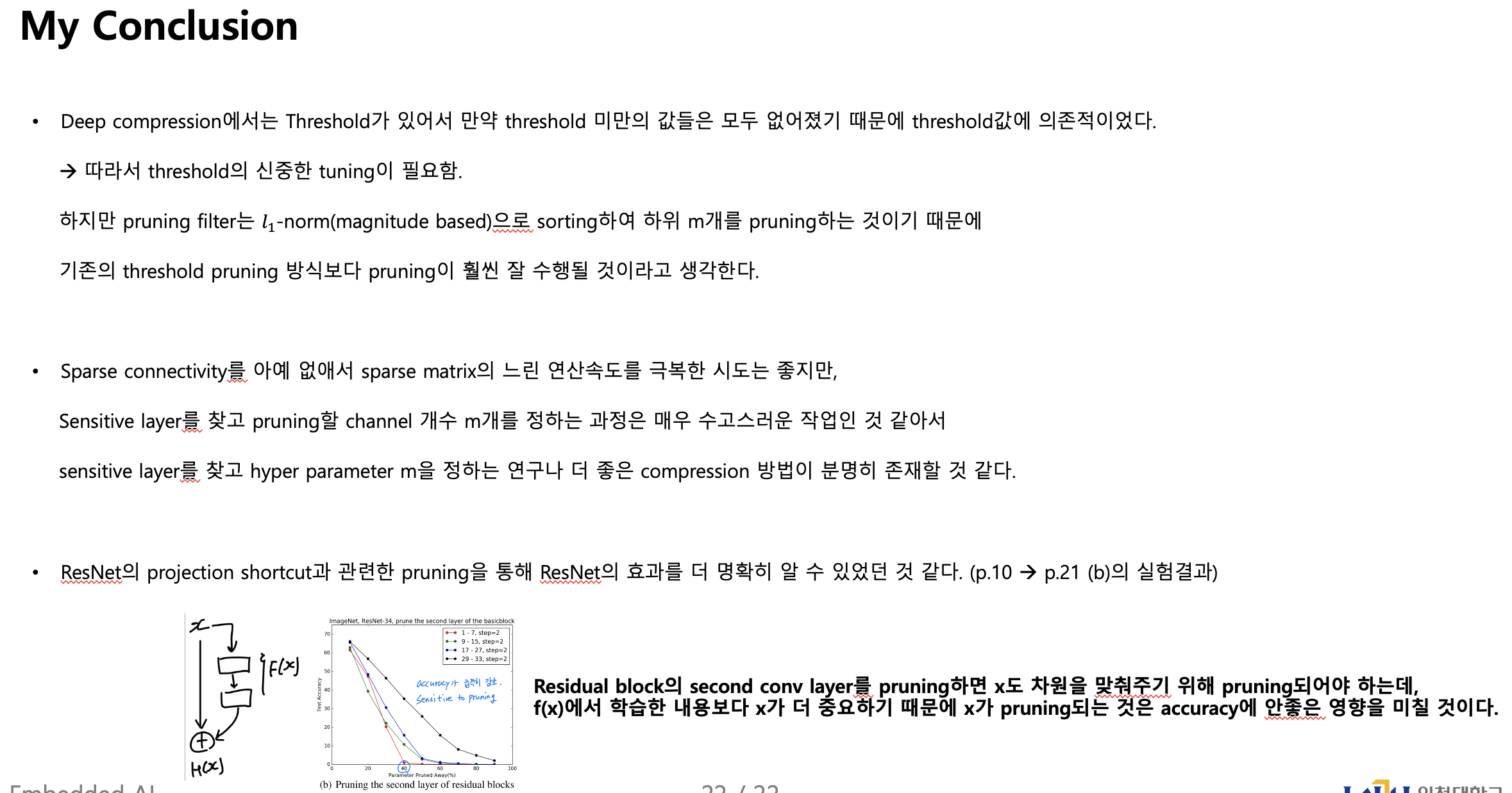
  문제는 second conv layer의 output feature map과 identity feature map을 대응시키는 데에서
  차원이 맞지 않아 prune에 어려움이 발생한다.
  그래서 residual block의 second conv layer를 prune하기 위해서는,
  proected feature map 또한 pruned되어야 한다.

3.4 Retraining Pruned Networks to Regain Accuracy

• filter를 pruning하고 난 뒤,
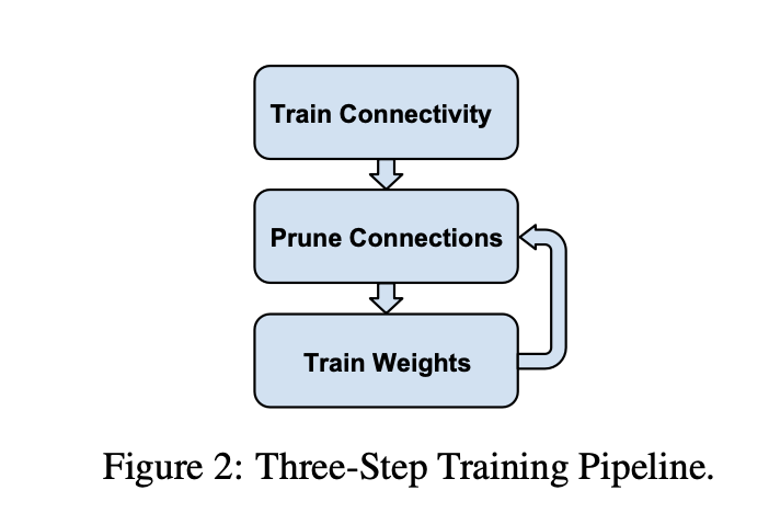
  performance degradation은 network를 retraining시켜줌으로써 보상되어질 수 있다.

  1. Prune once and retrain :
     multiple layers들의 filter들을 한번에 pruning하고, original accuracy로 복구될 때까지 retrain시킨다.
  2. Prune and retrain iteratively :
     layer by layer 또는 filter by filter로 filter들을 pruning하고, iteratively retrain시킨다.
     model은 pruning process에서 변경된 weight들을 적용하기 위해 다음 layer를 pruning하기 전에 retrain되진다.

• pruning에 resilient(회복력 있는) layer들의 경우,
  한번에 prune과 retrain하는 전략을 사용하여 network의 상당 부분을 제거할 수 있고,
  original training time 보다 더 적은 시간을 retraining함으로써 loss in accuracy를 회복할 수 있다.
  하지만,
  sensitive layer에 있는 몇가지 filter들이 pruned되거나 network의 상당 부분이 pruned 되어질 때,
  original accuracy를 복구하지 못 할 수도 있다.
  Iterative pruning and retraining은 더 좋은 결과를 내지만,
  very deep network에 대해서 훨씬 많은 epoch이 필요하다.

  정리
  1) Prune once and retrain 방식은
  retraining이 빠르지만 pruning에 sensitive한 layer들의 filter들이 pruning되어진다면,
  accuracy를 복구하지 못할 수도 있다.
  1) Prune and retrain iteratively 방식은
  retraining이 매우 느리지만 더 좋은 결과를 낼 수 있다.

---

4. Experiments

• 우리는 두가지 network type을 prune해봤다.
  1. simple CNNs(VGG-16 on CIFAR-10)
  2. Residual networks(ResNet-56/110 on CIFAR-10 and ResNet-34 on ImageNet)
• model compression을 설명하는 데에 자주 사용되는 AlexNet or VGG(on ImageNet)과는 다르게,
  VGG(on CIFAR-10) and Residual networks는 fully connected에 더 적은 parameter를 갖는다.
  그러므로 이렇게 FC layer에 parameter가 많은 network(AlexNet)들의 parameter를 pruning하는 것은 도전적이다.
  (내 생각 : filter를 pruning하는 기법이기 때문에 FC layer의 parameter가 많은 AlexNet과 같은 network들의 parameter수를 줄이는 것을 어려웠다고 주장하는 듯하다.)
  • AlexNet의 FC layer의 많은 parameters
    
  • ResNet의 Fc layer의 적은 parameters
    

• filter가 pruned되어질 때,
  더 적은 수의 filter를 갖는 새로운 model이 만들어지고,
  영향을 주지 않는 layer들 뿐만 아니라 변경된 layer들의 remaning parameter들은
  새로운 model에 copy되어 진다.
  
  게다가 만약 convolutional layer가 pruned되어진다면,
  다음의 batch normalization layer의 weight도 제거된다.

• 각 network의 baseline accuracy를 얻기 위해서,
  우리는 각 model from scratch를 train시켰고,
  ResNet과 똑같은 똑같은 pre-processing and hyperparameters를 사용했다.
  (model from scratch란?)

• retraining을 위해서,
  우리는 constant learning rate 0.01을 사용했고,
  original training epochs의 1/4만 진행시켰다.
  따라서 CIFAR-10에 대해서는 40 epochs를 retrain시켰고,
  ImageNet에 대해서 20 epochs을 train시켰다.

• VGG-16 : original VGG-16
  VGG-16-pruned-A : original VGG-16에 pruning하여 retraining
  VGG-16-pruend-A scratch-train : original VGG-16에 pruning한 model을 처음부터 다시 training
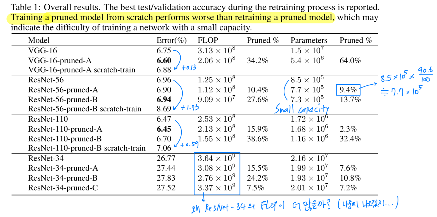
  Table 1에서 볼 수 있듯이,
  training a pruned model from scratch가 retraining a pruned model보다 성능이 낮은 것을 알 수 있다.
  그리고 training a pruned model from scratch는 small capacity network에 training 되는 것에 어려움이 있다.

4.1 VGG-16 on CIFAR-10

• VGG-16은 원래 ImageNet dataset을 위해 design된 high-capacity network이다.
  최근에 Sergey Zagoruyko(2015)는 CIFAR-10에 맞게 살짝 수정된 VGG-16 version을 공개했고, state of the art result를 달성했다.
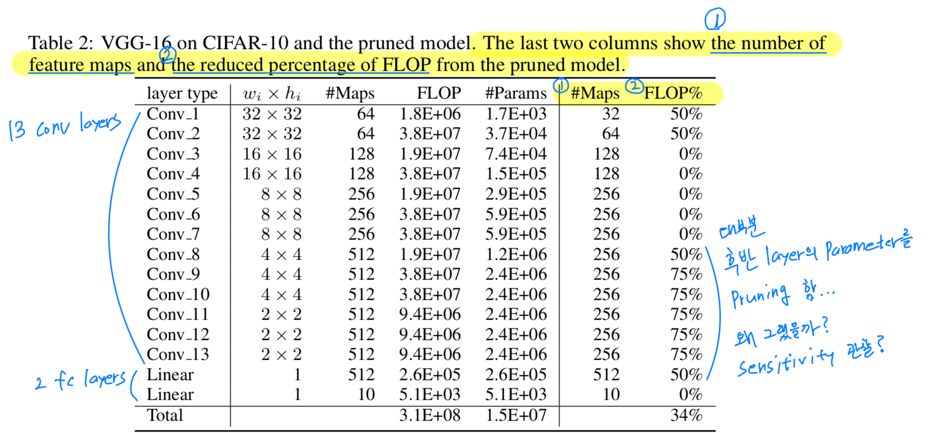  Table 2에서 볼 수 있듯이, CIFAR-10에 대한 VGG-16은
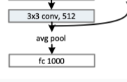
  13개 conv layer와 2개의 fc layer로 구성되어 있고,
  fc layer는 small input size와 less hidden units으로 인해 parameter의 많은 부분을 차지하지 않는다.
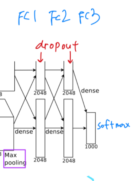
  우리는 Sergey Zagoruyko(2015)가 제안한 model을 사용했지만,
  모든 conv layer 이후 activation과 첫번째 linear layer에 Batch Normalization을 적용했고,
  dropout은 사용하지 않았다.
  (last conv layer가 pruned된다면, linear layer의 input도 바뀌고 connection이 제거된다는 것을 명심하자)

• Figure 2(b)에서 볼 수 있듯이,
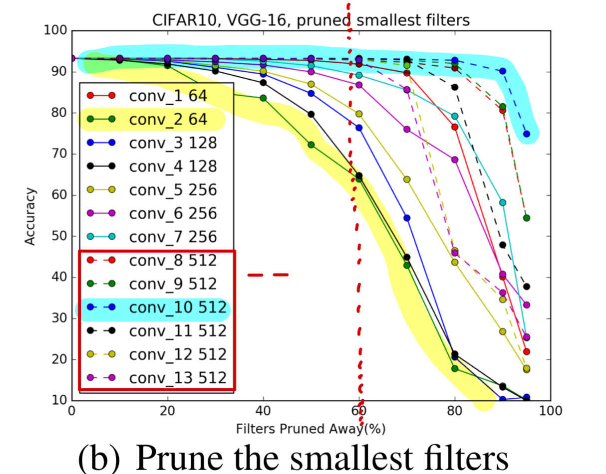  512개의 feature map을 가진 convolutional layer들은
  accuracy에 영향 없이 적어도 60%의 filter를 drop할 수 있다.
  
  Figure 2(c)에서는 retraining에 대한 것을 보여준다.
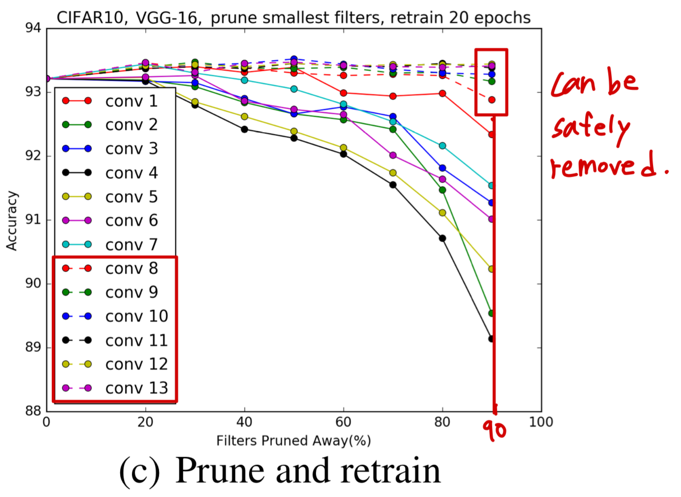  512개의 feature map을 가진 convolutional layer들의 거의 90%의 filter들은 안전하게 제거될 수 있다.
  
  이에 대한 한가지 가능한 설명으로는
  512개의 feature map을 가진 convolutional layer의 filter들은
  4x4 or 2x2 feature map에서 동작한다는 것이며,
  이는 small dimension에서 meaninful spatial connection을 갖고 있지 않을 것이라고 생각할 수 있다.
  예를 들어, CIFAR-10에 대한 ResNet은 8x8 dimension 밑으로 된 feature map을 사용하지 않는다.
  우리는 first layer가 다른 layer들에 비해 pruning에 robust하다는 것을 발견했다.
  = (내 해석) first layer의 pruning sensitivity가 낮다
  이것은 CIFAR-10과 같이 simple dataset에 대해서 가능하며,
  ImageNet과 같은 큰 dataset에 대해서는 그렇게 useful filter들을 학습하지 않는다.(Figure. 5)
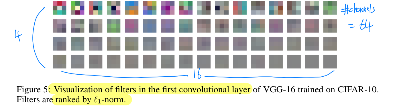  만약 first layer filter의 80%를 pruned한다면,
  남아있는 filter는 12개($64 * 0.8 = 12$)인데,
  12개는 the number of raw input channels(3)보다 여전히 크다.
  하지만,
  second layer로부터 80%의 filter를 pruned한다면,
  second layer에서도 64에서 12개로 mapping이 될텐데,
  이는 first layer로부터 significant information을 잃는 것일지도 모른다.
  그래서 accuracy에 손해가 있을 것이다.
  ➡️ 내 해석 : 초기 layer에 너무 많이 pruning을 한다면, raw data information을 많이 잃을 수 있어서 좋지 않을 것이다.
  
  그래서 layer 1의 filter pruning을 50%로 하고,
  layer 8 ~ layer 13의 filter pruning을 50%, 75%로 했을 때,
  우리는 같은 accuracy에 34% FLOP reduction을 달성할 수 있었다.

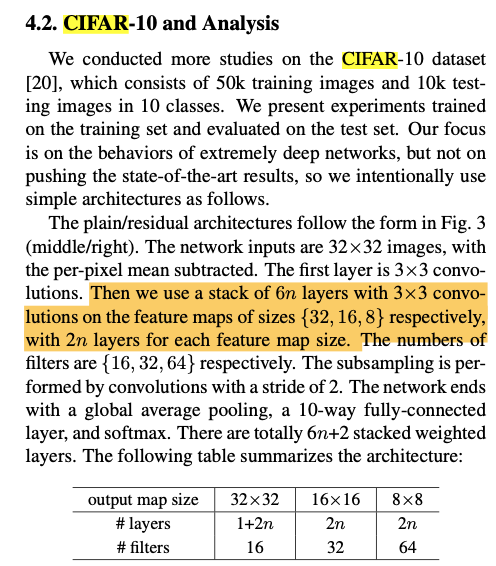
4.2 ResNet-56/110 On CIFAR-10

• ResNets for CIFAR-19은 feature map size가 32 x 32, 16 x 16, 8 x 8,
  이 3개의 stage를 갖는 residual block이 있다.
  각 stage는 똑같은 residual block 개수를 갖는다.
  feature map의 개수가 증가할 때,
  shourtcut layer는 increased dimension에 대한 추가적인 zero padding으로 identity mapping을 제공한다.
  identity feature map을 선택하는 projection mapping이 없기 때문에
  우리는 residual block의 첫번째 layer를 pruning하는 것만 고려했다.
  내 해석 :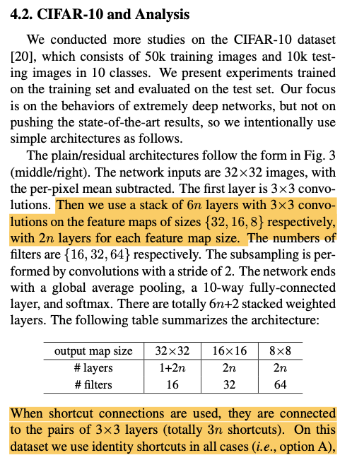 위와 같은 projection mapping이 없고 그냥 zero padding만 해서
  모든 경우에 identity shortcut이었기 때문에 first conv layer에 대해서만 pruning을 고려했다.

• Figure 6에서 볼 수 있듯이,
  대부분의 Layer는 pruning에 robust하다.
  
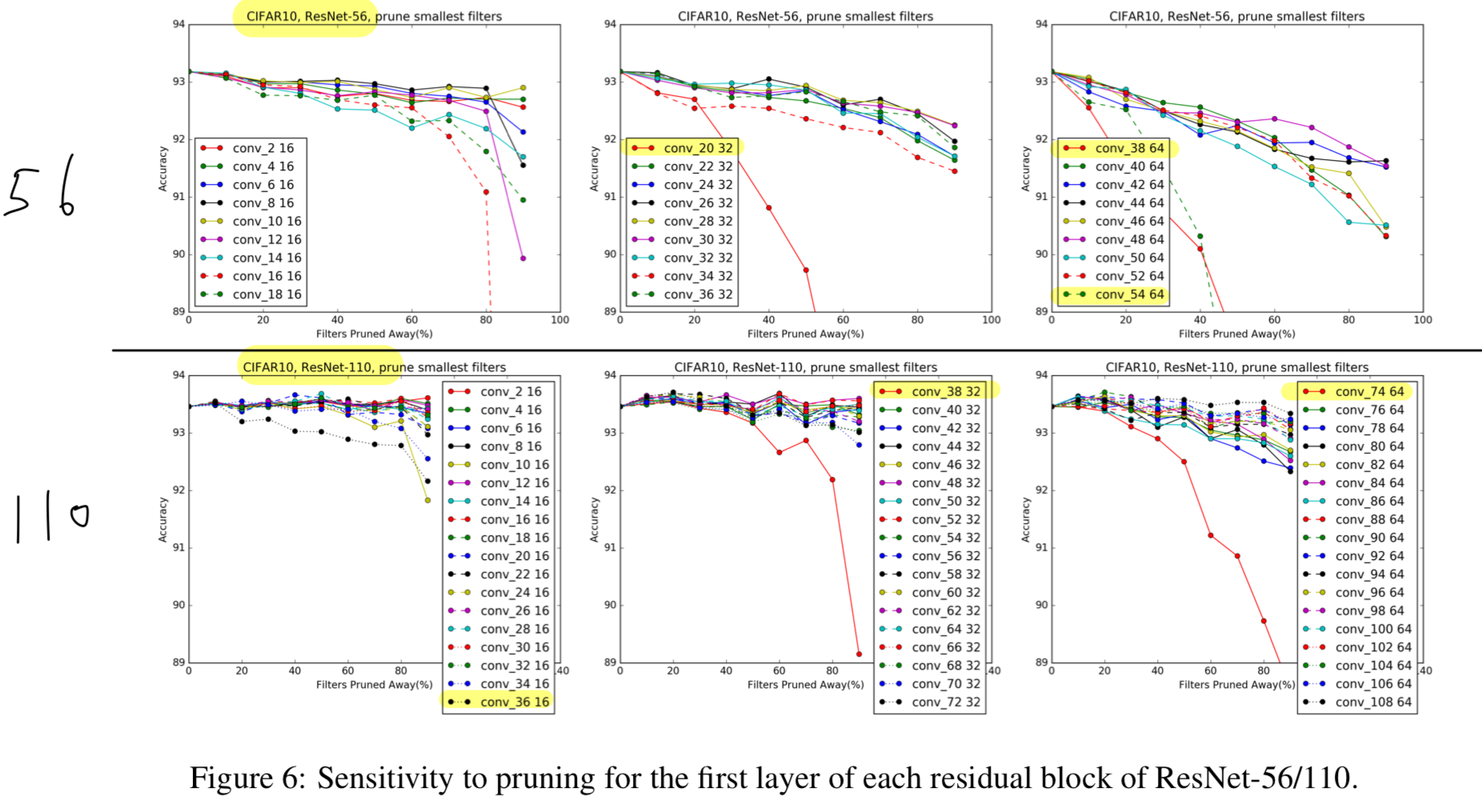
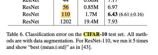
  ResNet-110에 대해서는,
  retraining 없이 some single layer를 pruning하는 것은 심지어 performance를 향상시켰다.
  추가로, 우리는 pruning에 sensitive한 layer
  (ResNet-56에서는 layer 20, 38, 54), (ResNet-110에서는 layer 36, 38, 74)
  들이 feature map의 개수가 변화하는 residual block에 있다는 것을 알아냈습니다.
  우리는 이것이 새롭게 추가되는 empty feature map에 대한 residual error가 필요하기 때문에 발생한다고 생각한다.

• retraining performance는 이러한 sensitive layer들을 skip함으로써 향상될 수 있다.
  Table 1에서 볼 수 있듯이,
  ResNet-56-pruned-A는 sensitive layer 16, 20, 38, 54를 skip하여,
  10%의 filter를 pruning함으로써 accuracy를 향상시켰다.
  게다가 우리는 deeper layer들이 earlier layer들보다 더욱 pruning에 sensitive하다는 것을 알아냈다.
  그래서, 우리는 각 stage마다 다른 pruning rate를 사용했다.
  
  우리는 $i$th stage에 대한 layer에 pruning rate를 $p_i$로 denote하여 사용할 것이다.
  
  ResNet-56-pruned-B는 더 많은 layer들(16, 18, 20, 34, 38, 54)을 skip 했고,
  $p_1=60$, $p_2=30$, $p_3=10$로 layer를 pruning했다.
  
  ResNet-110에 대해서는,
  ResNet-110-pruned-A model에 대해서는 $p_1=50$와 layer 36을 skip하는 것이 살짝 더 좋은 결과가 있었다.
  ResNet-110-pruned-B model에 대해서는 layer 36, 38, 74를 skip 했고,
  $p_1=50$, $p_2=40$, $p_3=30$로 layer를 pruning했다.
  
  만약 각 stage에 2개의 residual block보다 더 많이 있다면,
  가운데에 있는 residual blcok이 redundant되었고, pruned하기 더 쉬울 것이다.
  이것이 왜 ResNet-110이 ResNet-56보다 pruning하기 더 쉬운 이유가 될 것이다.

4.3 ResNet-34 On ILSVRC2012

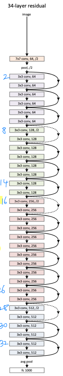
• ImageNet을 위한 ResNet은 56 x 56, 28 x 28, 14 x 14, 7 x 7
  이 4개의 stage를 갖는 residual block이 있다.
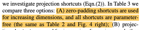
  ResNet-34는 feature map이 down-sampled될 때, projection shortcut을 사용한다.
  
  (내 생각)
  ResNet-56/110은 weight에 zero padding을 해서 identity mapping을 수행했었는데,
  ResNet-34는 projection shortcut($W_s$)을 사용했기 때문에 ResNet-56/110보다 parameter 개수가 더 많은것인가?
  하지만 그렇다고 하더라도 projection shortcut은 1x1 kernel일텐데 layer가 훨씬 더 깊은 ResNet-56/110보다 parameter가 더 많은게 말이 안된다...
  ResNet-34의 parameter가 더 많은 것은 아직도 잘 모르겠다.
  (내 생각)
  ResNet-56/110은 CIFAR-10 dataset을 사용했으니까 FLOP, parameter수가 훨씬 적은 것임.
  ResNet-34는 CIFAR-10보다 더 큰 ImageNet dataset을 사용했으니까 layer가 훨씬 적더라도 FLOP, parameter수가 훨씬 큰 것임.
  (궁금증)
  그럼 왜 ResNet-56/110은 CIFAR-10에 실험하고, ResNet-34는 ImageNet에 실험했을까?
  ResNet 논문에서 그렇게 했음...
  

• 우리는 첫번째로 각 residual block의 first layer를 prune했다.
  Figure 7에서는 각 residual block의 first layer의 sensitivity를 보여준다.
  ResNet-56/110과 유사하게,
  각 stage의 the first and the last residual block(layer 2, 8, 14, 16, 26, 28, 30, 32)은
  itermediate block보다 pruning에 더욱 sensitive하다.
  따라서 우리는 이러한 layer들을 skip했고,
  각 stage에 남아있는 layer들을 동등하게 pruning하였다.
  
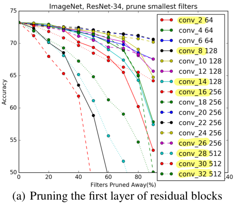
  (a) : layer 2, 8, 14, 16, 26, 28, 30, 32 은 sensitive하기 때문에 skip함.
  
  Table 1에서,
  우리는 처음 3개의 stage(56 x 56, 28 x 28, 14 x 14)에 대한
  pruning percentages의 2가지 configuration에 대해서 비교했다.
  (A) = ResNet-34-pruned-A : $p_1=30$, $p_2=30$, $p_3=30$
  (B) = ResNet-34-pruned-B: $p_1=50$, $p_2=60$, $p_3=40$
  (C) = ResNet-34-pruned-C: $p_1=30$, $p_2=30$, $p_3=20$
  option (B)는 약 1%의 accuracy loss로 24%의 FLOP reduction을 제공한다.
  ResNet-56/110에 대한 pruning result에서 볼 수 있듯이,
  우리는 ResNet-34가 deeper ResNet과 비교하여 상대적으로 더욱 prune하기에 어려울 것이라고 생각할 수 있었다.

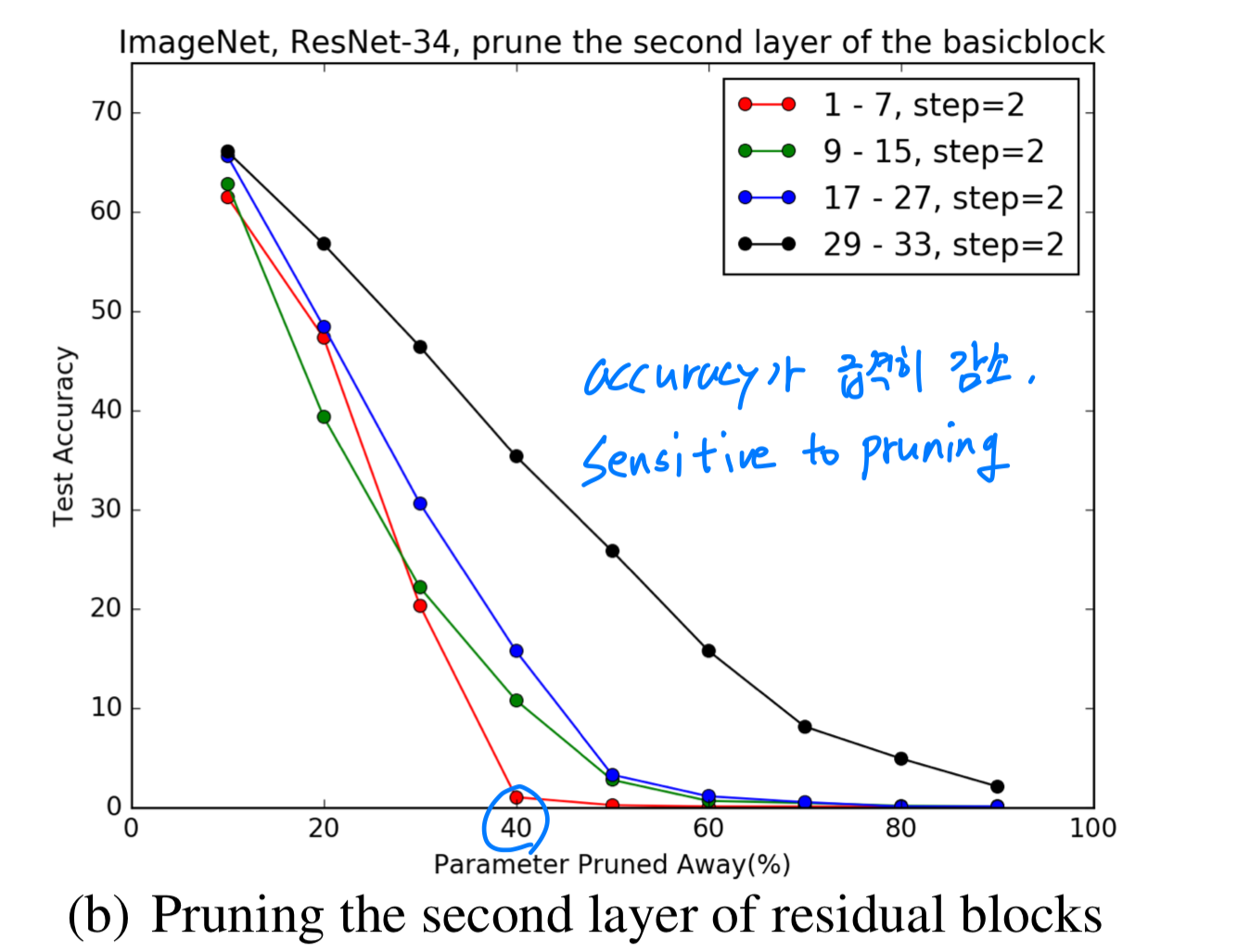
• 우리는 또한 identity shortcut와 residual block의 second conv layer를 pruning해봤다.
  이 layer들은 같은 filter 개수를 갖기 때문에, 동등하게 pruned되어졌다.
  Figure 7(b)에서 볼 수 있듯이,
  이러한 layer들은 first layer들보다 pruning에 더욱 sensitive하다.
  retraining하여, ResNet-34-pruned-C를 $p_3=20$로 pruning한 결과,
  accuracy에 0.75% 손해를 보고 7.5% FLOP reduction을 했다.
  그러므로 residual block의 first layer를 pruning하는 것이 second layer를 pruning하는 것보다 overall FLOP을 줄이는 데에 훨씬 효과적이다.
  

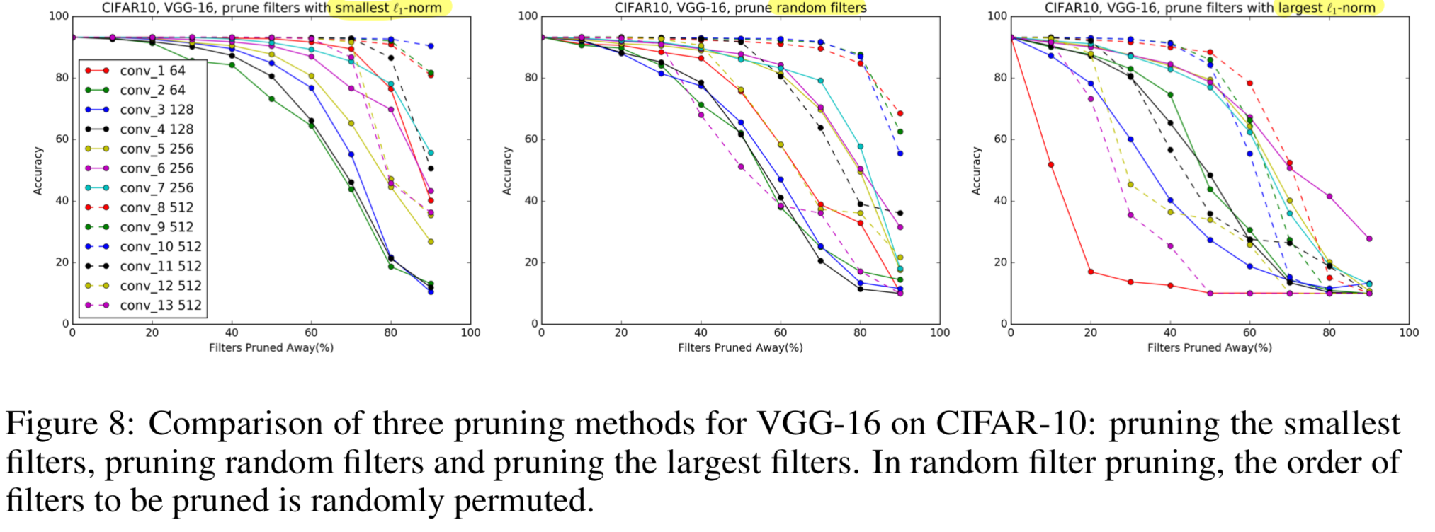
4.4 Comparison with pruning random filters and largest filters

• 우리는 random filter를 pruning하는 것과 largest filter를 pruning하는 것을 비교해봤다.
  Figure 8에서 볼 수 있듯이,
  smallest filter에 pruning을 적용하는 것은
  대부분의 layer에 각각 다른 pruning ratio로 random filter를 pruning하는 것보다
  성능이 좋게 나온다.
  largest $l_1$-norm을 가진 filter를 pruning하는 방법의 accuracy는 pruning ratio를 증가시킬수록 급격히 떨어지고,
  이것은 larger $l_1$-norm을 갖는 filter의 중요도를 설명하게 된다.
  

4.5 Comparison with activation-based feature map pruning

• The activation-based feature map pruning method는
  weak activation pattern과 그에 해당하는 filter와 kernel에 대한 feature map을 제거하는 방법으로,
  어떤 feature map을 pruning할 것인지 결정하기 위한 input으로 sample data가 필요하다.
  여기서 우리는 batch normalization 이나 non-linear activation을 거지기 전인 convolution operation으로부터 feature maps에 대한 statistic을 계산했다.
  (왜 이렇게 계산했을까?
  내 생각 : BN에서 mean, std를 일정하게 정규화하니까 비교가 정확하지 않을 수 있기 때문인 듯하다.
  그리고 non-linearity를 거치면서 mean, std가 극적으로 변하니까 비교가 정확하지 않을 수 있기때문인 듯하다)
  우리는 $l_1$-norm based filter pruning과 다음의 방법들을 비교해봤다.
  
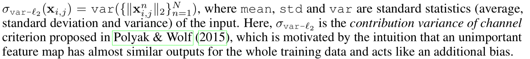
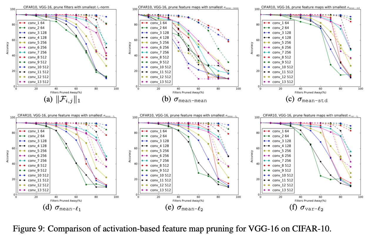
  ➡️ $\sigma_{mean-std}$ criterion이 pruning ratio of 60%일 때까지 $l_1$-norm 방식과 비슷한 performance를 보이거나 더 좋은 모습을 보였다.
  하지만 특히 conv 1, conv 2, conv 3 layer에서 performance가 급격히 떨어졌다.
  우리는 $l_1$-norm criterion이 filter selection considering에 좋은 heuristic이라는 것을 알아냈다.

---

5. Conclusions

• Modern CNNs은 보통 large training and inference costs로 high capacity를 갖는다.
  이 논문에서 우리는 irregular sparsity 없이 computation cost를 제거할 수 있는 CNNs을 만들기 위해
  상대적으로 작은 weight magnitude를 갖는 filter를 pruning하는 방법을 소개했다.
  우리는 one-shot pruning과 구현하기 쉬운 retraining strategy를 사용했다.
  very deep CNNs에 대한 매우 힘들었던 연구를 수행함으로써,
  우리는 pruning에 robust하거나 sensitive한 layer들을 찾을 수 있었고,
  이러한 실험은 acrhitecture를 이해하고 발전시키는 데에 유용할 것이다.

My Conclusion

---

궁금한 점, 모르겠는 점

• the number of operations, computational cost의 정확한 정의와 각각의 계산원리를 모르겠다..
  

• FLOPs vs MACs ?

  • FLOPS :
    FLoating point OPerations per Second
    1초 동안 얼마나 많은 floating point operation을 하는지에 대한 지표.
    보통 컴퓨터의 성능을 나타내는 데에 주로 사용되나,
  • FLOPs :
    FLoating point OPerations.
    딥러닝에서의 FLOPS는 단위 시간이 아닌 절대적인 연산량
    (addition, subtraction, multiplication, and division)의 횟수를 지칭.
    $a*x + b$ 에서
    FLOPs = 2 ➡️ $a*x$, + b
  • MACs :
    Multiply-ACcumulate operations.
    multiplying two numbers and adding the result.
    이 연산은 matrix multiplications, convolutions, dot products와 같이
    두 수를 곱하고 더하는 연산이 있는 linear algebra operations에 많이 사용된다.
    $a*x + b$ 에서
    MACs = 1 ➡️ $(a*x + b)$

    일반적으로
    FLOPs : MACs = 2 : 1
    100MACs = 200FLOPs
    100FLOPs = 50MACs

• ResNets for CIFAR-10 model 정보는 ResNet 논문에서 찾을 수 있었다.
  

• 그럼 VGG-16 on CIFAR-10에서 small dimension filter(4x4, 2x2)들을 조금 더 큰 dimension으로 키웠다면,