Paper Info

NeurIPS 2021

---

Abstract

• Sparsely-gated MoEs networks는 NLP에서 excellent scalability를 입증해왔다.
  하지만 Computer Vision에서, 모든 performant networks는 "dense"하다.
  즉, every input이 every parameter에 의해 processed된다.
  우리는 largest dense networks에 대한 scalable and competitve한
  a sparse version of the Vision Transformer인, a Vision MoE (V-MoE)를 소개한다.

• image recognition에 적용했을 때, V-MoE는 SOTA network와 performance가 동등하면서도 inference 시 computation을 절반까지 줄일 수 있다.
  추가로, 우리는 routing algorithm을 확장하여 entire batch에서 each input의 subsets을 prioritize(우선 처리)할 수 있는 방식을 제안하며,
  이를 통해 adaptive per-image compute를 할 수 있다.
  이를 통해 V-MoE는 test 시 performance와 computation 간의 trade-off를 smoothly하게 만들 수 있다.
  마지막으로, 우리는 vision models을 확장하기 위한 V-MoE의 가능성을 입증하며, 15B parameter model을 train하여 ImageNet에서 90.35%의 성능을 달성했다.

---

1 Introduction

(network capacity 증가로, high computational cost가 요구되고 있음...)

• DL은 역사적으로 network capacity and dataset size를 증가시키면 performance가 향상된다는 사실이 증명되었다.
  CV나 NLP에서 이러한 방법으로 SOTA를 자주 달성해 왔다.
  그러나 이러한 models을 training하고 serving하는 것은 expensive하다.
  이는 부분적으로 deep networks가 일반적으로 "dense"하기 때문이다 - 즉, every example이 every parameter를 사용하여 processed되므로 scale이 커질수록 high computational cost를 요구한다.

(NLP에서 conditional computation은 위 문제를 해결하려는 접근법임)

• 반면, conditional computation은 각 example에 대해 only a subset of parameters만 적용하여
  model capacity를 증가시키면서도 training and inference cost를 대체로 constant(일정하게) 유지하려고 한다.
  NLP에서는 sparse MoEs가 점점 인기를 얻고 있으며, 이를 통해 trillion parameter models을 training and inference에 필요한 resource를 줄일 수 있게 한다.

(우리는 ViT를 사용하여 conditional computation을 vision에 대해 확장하려고 한다)

• 이 연구에서, 우리는 conditional computation for vision at scale을 탐구한다.
  우리는 image classification을 위한 Vision MoE (V-MoE)를 소개하며, 이는 최근의 ViT architecture의 a sparse variant이다.
  V-MoE는 a subset of the dense feedforward layers in ViT를 sparse MoE layers로 대체하며,
  여기서 각 image patch는 a subset of "experts" (MLPs)로 "routed"된다.

(기존 routing network의 non-differentiability를 개선한 학습 방법을 제안했다)

• 하지만 unique(고유한) failure modes and non-differentiability로 인해 deep sparse models에서 routing은 challenging하다.
  우리는 다양한 design choices를 탐구하고, V-MoE의 pre-training and transfer를 위한 effective recipe를 제시하며, 특히 dense counterpart보다 우수한 성능을 달성했다.

(inference 동안 sparsity level을 조절함으로써 performance vs. inference-cost trade-off를 조절할 수 있다)

• 또한 V-MoE models이 매우 flexible한 것을 보여준다.
  already trained models의 performance vs. inference-cost trade-off는
  input and/or the model weights의 sparsity level을 조절함으로써 inference 동안에 smoothly adjusted될 수 있다.
  V-MoE를 통해 model sizes of 15B params로 확장할 수 있으며, 이는 largest vision models to date(현재까지)이다.
  우리는 SOTA dense models의 성능과 동등한 수준을 달성하면서도 fewer time to train을 필요로 한다.
  또는 V-MoE는 the cost of ViT에 맞추면서 better performance를 제공할 수 있다.
  이러한 tradeoff를 제공하기 위해, 우리는 Batch Prioritized Routing을 제안한다.
  이 routing algorithm은 model sparsity를 활용하여 the computation of some patches을 skip하여, uninformative image regions에서 computation을 줄인다.

• our main contributions을 다음과 같이 요약:

  • Vision models at scale.(확장 가능한 vision models)
    우리는 V-MoE라는 distributed sparsely-activated Transformer model for vision을 제시한다.
    최대 24개 MoE layers, 32 experts per layer, and almost 15B params를 가진 model을 train했다.
    이러한 models은 stably trained될 수 있으며, transfer에 무리 없이 사용되고, 최소 1000개의 datapoints만으로도 성공적으로 fine-tuned된다는 것을 보여줬다.
    (datapoints가 뭐지? -> ImageNet-21k에서 pre-trained model을 새로운 task에 대한 1000개의 data만으로도 성공적인 fine-tuning이 된다는 의미인듯)
  • Performance and inference.
    V-MoE는 dense counterparts 대비 절대적으로 outperform하며, upstream, few-shot and full fine-tuning metrics에서 두드러지는 결과를 보인다.
    또한, inference 시 V-MoE은 largest dense model's performance를 만족하면서도 절반 이하의 computation 또는 actual runtime, 또는 same cost로 outperform할 수 있도록 조정할 수 있다.
  • Batch Prioritized Routing.
    우리는 V-MoE에서 least useful patches를 discard할 수 있도록 하여 각 image에 대한 computation을 줄일 수 있는 a new priority-based routing algorithm을 제안한다.
    특히, 우리는 V-MoEs가 training FLOPs의 20%를 절약하면서도 dense models의 performance를 유지할 수 있음을 보여준다.
  • Analysis.
    우리는 some visualization of routing decisions을 제공하며, 이는 우리가 design decisions을 motivate했던 patterns and conclusiosn을 보여준다.
    이는 이 field에 대한 이해를 발전시키는 데에 기여할 수 있다.

---

2 The Vision Mixture of Experts

• 첫번째로 MoEs and sparse MoEs에 대해 설명할 것이다.
  그리고나서 어떻게 우리가 이 methodology를 vision에 적용했는지 설명하고,
  routing algorithm을 위한 design choices와 V-MoEs의 implementation을 설명할 것이다.

2.1 (사전 지식) Conditional Computation with MoEs

• Conditional computation은 서로 다른 inputs에 대해 network의 서로 다른 subsets을 활성화하는 것을 목표로 한다.
  mixture-of-experts model은 specific instantiation(특정 구현) 방식으로, 서로 다른 model "experts"들이 inpput space의 서로 다른 regions을 담당한다.
  우리는 [54]의 setting을 따르며, $E$개의 experts를 가진 a mixture of experts layer를 다음과 같이 정의한다:
  $MoE(x)=\Sigma^{E}_{i=1}g(x)_ie_i(x)$
  where $x \in \R^D$ is the input to the layer,
  $e_i : \R^D \to \R^D$ is the function computed by expert $i$,
  and $g : \R^D \to \R^E$ is the "routing" function which prescribes the input-conditioned weight for the experts.
  $e_i$ and $g$는 모두 neural network로 parameterized된다.

• 이 정의에 따르면, 이는 여전히 dense network이다.
  그러나 $g$가 sparse하다면, 즉 $k << E$의 non-zero weights만 assign되도록 제한된다면, unused experts는 computed될 필요가 없다.
  이는 inference and training computation에 비해 model의 #params을 super-linear scaling(초선형적인 확장)을 할 수 있도록 해준다.

  • 궁금한 점 :
    [54]에서 gating network $g$는 sparse하지 않나?
    Noisy Top-K Gating으로 k값을 조정하면서 sparsity를 제어하는 걸로 이해했는데...
    

2.2 (제안) MoEs for Vision

• 우리는 ViT 맥락에서 sparsity를 vision에 적용하는 것을 탐구했다.
  ViT는 transfer learning setting에서 잘 확장되는 것으로 입증되었으며, CNN보다 적은 pre-training compute로 better accuracies를 달성한다.

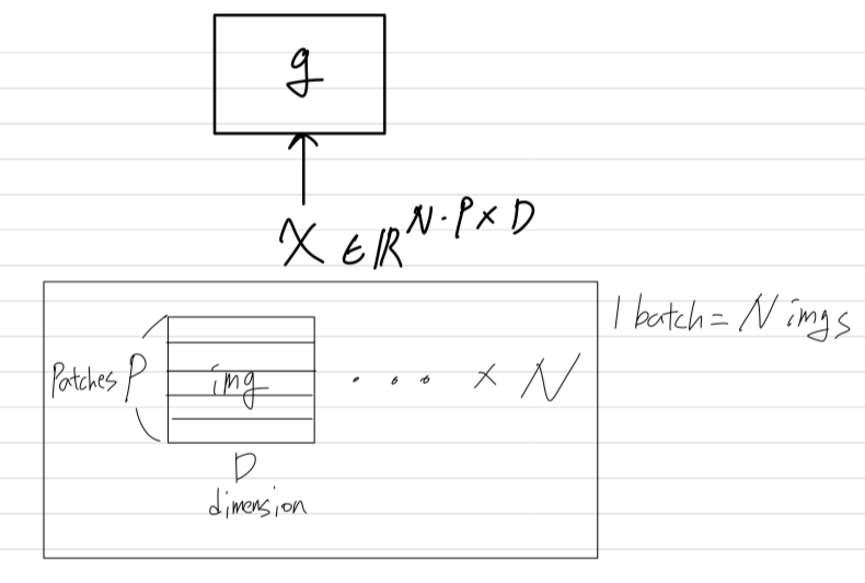
• ViT는 images를 a sequene of patches로 처리한다.
  input image는 먼저 equal-sized patches로 구성된 grid로 divided된다.
  그런 다음 이를 Transformer's hidden size로 linearly projected된다.
  이후 positional embedding을 추가한 후, patch embeddings(tokens)은 주로 self-attention and MLP layers가 교차하는 Transformer에 의해 처리된다.
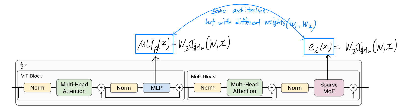
  MLP는 two layers and a GeLU non-linearity를 사용하여 정의된다: $MLP(x) = W_2\sigma_{gelu}(W_1x)$
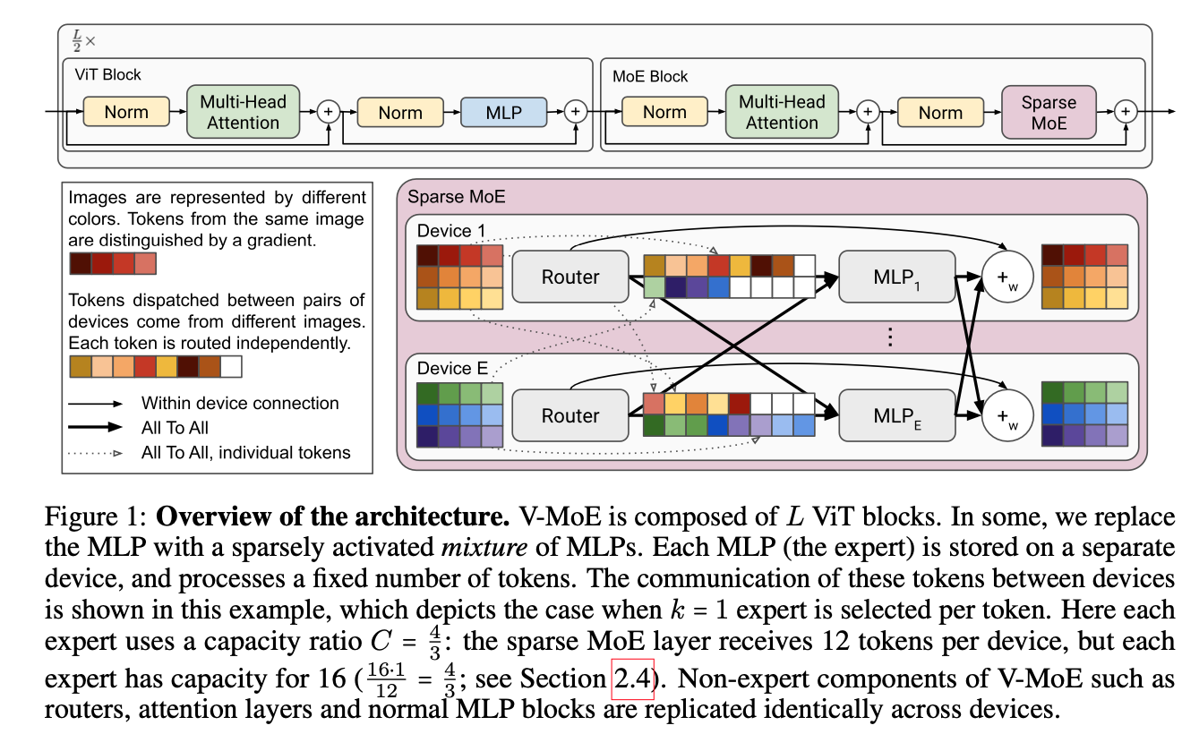
  Vision MoE에서는 이러한 MLP layer 중 subset을 MoE layers로 교체하며, 각 expert는 MLP이다. (Figure 1)
  experts는 $e_i(x) = MLP_{\theta_i}(x)$와 same architecture를 가지지만 different weights $\theta_i=(W_1^i, W_2^i)$를 갖는다.
  이는 M4 machine translation model의 design pattern과 유사하다.
  

2.3 (제안) Routing

• V-MoE의 각 MoE layer에서 routing function $g(x) = TOP_k(softmax(Wx+\epsilon))$을 사용했다,
  where $TOP_k$는 vector의 모든 elements 중 largest $k$ values를 제외한 나머지를 모두 0으로 만드는 연산,
  and $\epsilon$은 $\epsilon$ ~ $N(0, \frac{1}{E^2})$ entry-wise마다 독립적으로 sampled된다. (MoE 논문에서 추가한 Gaussian noise인듯)
  실제로, 우리는 $k=1$ or $k=2$를 사용했다.
  ViT의 맥락에서, $x$는 network의 특정 layer에서 image token의 representation을 나타낸다.
  따라서, V-MoE는 entire images를 routing하는 것이 아니라 patch representations을 routing한다.

• 이전 formulations [54]과의 차이점은 experts weights에 대해 softmax 이후에 $TOP_k$를 적용한다는 것이다.
  이는 softmax 이전에 $TOP_k$를 적용했을 때의 문제(rounting에 대한 gradients가 거의 모든 곳에서 0이 되는 현상)을 방지하며, $k>1$일 때도 더 나은 성능을 보인다(Appendix A).

  • 이전 formulations [54] :
    $g(x) = softmax(TOP_k(Wx+\epsilon))$
  • 이 논문의 formulations (softmax와 $TOP_k$의 위치 바꿈)
    $g(x) = TOP_k(softmax(Wx+\epsilon))$

(아래는 이전 논문 [54]에서 했던 방법을 그대로 사용)

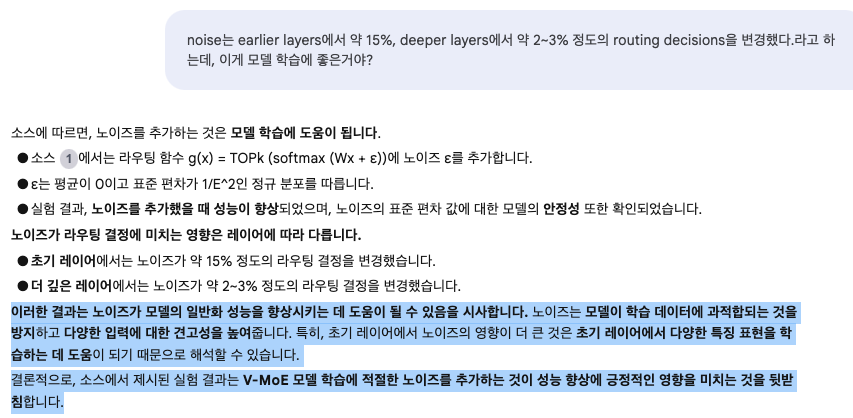
• 마지막으로 우리는 activations $Wx$에 a small amount of noise with standard deviation $\frac{1}{E}$를 추가했다.
  $(Wx + \epsilon$ ~ $N(0, \frac{1}{E^2}))$
  실험적으로 이 setting이 잘 작동함을 확인했으며, 이 parameter에 대해 setup이 비교적 robust함을 발견했다.
  noise는 earlier layers에서 약 15%, deeper layers에서 약 2~3% 정도의 routing decisions을 변경했다.
  • 궁금한 점 : noise가 routing decision을 변경하면 좋은 건가?
    특정 expert만 specialized되는 문제(overfitting)를 방지할 수 있는 듯함.
    

2.4 (제안) Expert’s Buffer Capacity

(그냥 training하면 다음과 같은 문제들 발생...)

• training 동안 sparse models은 only a small set of experts만 선호하는 경향이 있다.
  이러한 common failure mode는 two problems을 초래할 수 있다.
  1. statistical inefficiency:
     a single expert로 수렴할 경우, model은 더 이상 dense model보다 powerful하지 않는다.
  2. computational inefficiency:
     imbalanced assignments of items to experts는 poor HW utilization을 유도한다.

(문제를 해결하기 위한 load balancing 방법 제시)

• 이러한 imbalance를 해결하고 implementation을 단순화하기 위해,
  우리는 각 expert의 buffer capacity(각 expert가 처리할 수 있는 #tokens)를 고정시키고,
  load balancing을 encourage하는 auxiliary losses를 추가하여 model을 train했다.
  이는 [54, 39, 22]에서 제안한 two of the auxiliary losses의 slight variants(약간 변형된 버전)를 사용한다.(Appendix A)

• expert의 buffer capacity $B_e$는
  batch에 포함된 #images $N$,
  #tokens per image $P$,
  #(selected experts per token) $k$,
  total #experts $E$,
  and the capacity ratio $C$로 정의된다:
  

• 만약 router가 어떤 expert에 대해 $B_e$이상의 token을 assign하면, $B_e$까지만 processed된다.
  나머지 tokens은 완전히 'lost'(손실)되지는 않으며, residual connections에 의해 그들의 information이 유지된다.
  또한 $k > 1$인 경우, 여러 experts가 각각의 token을 처리하려 시도한다.
  따라서 token이 완전히 discarded되지는 않는다.
  반대로, 특정 expert에게 할당된 token이 $B_e$보다 적을 경우, 나머지 buffer는 zero-padded된다.

• 우리는 capacity ratio $C$를 사용하여 the capacity of the experts를 조정했다.
  $C > 1$인 경우, routing imbalance를 고려하여 slack(여유) capacity를 추가했다.
  이는 new data가 upstream training(사전 훈련) 동안의 data distribution과 크게 다를 수 있는 fine-tuning 시유용하다.
  $C < 1$인 경우, router는 some assignmetns를 무시하도록 강제된다.
  Section 4에서는 $C << 1$로 설정하여 the least useful tokens을 버리고 inference 중 computation을 절약하는 a new algorithm을 제안한다.

---

3 Transfer Learning

(skip)

---

4 Skipping Tokens with Batch Prioritized Routing

• 우리는 model이 important tokens을 prioritize할 수 있도록 하는 a new routing algorithm을 제안한다.
  각 expert의 capacity를 동시에 줄임으로써 the least useful tokens을 discard할 수 있다.
  직관적으로, 모든 patch가 주어진 image를 classify하는 데 동일하게 중요한 것은 아니며,
  예를 들어, 대부분의 background patches는 model이 relevant entities(관련 있는 entities)가 있는 patch에만 집중하도록 하여 제거될 수 있다.

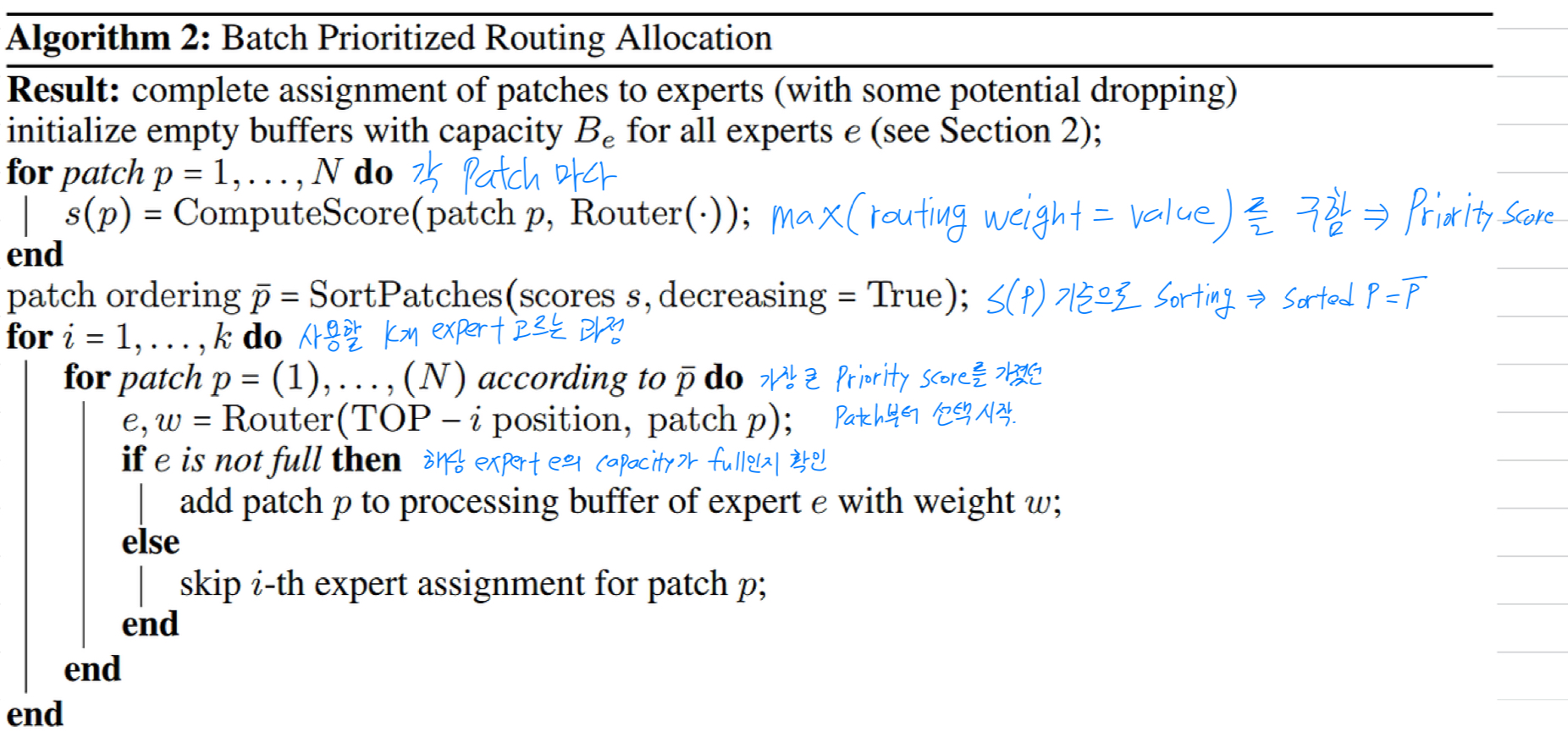
4.1 From Vanilla Routing to Batch Prioritized Routing

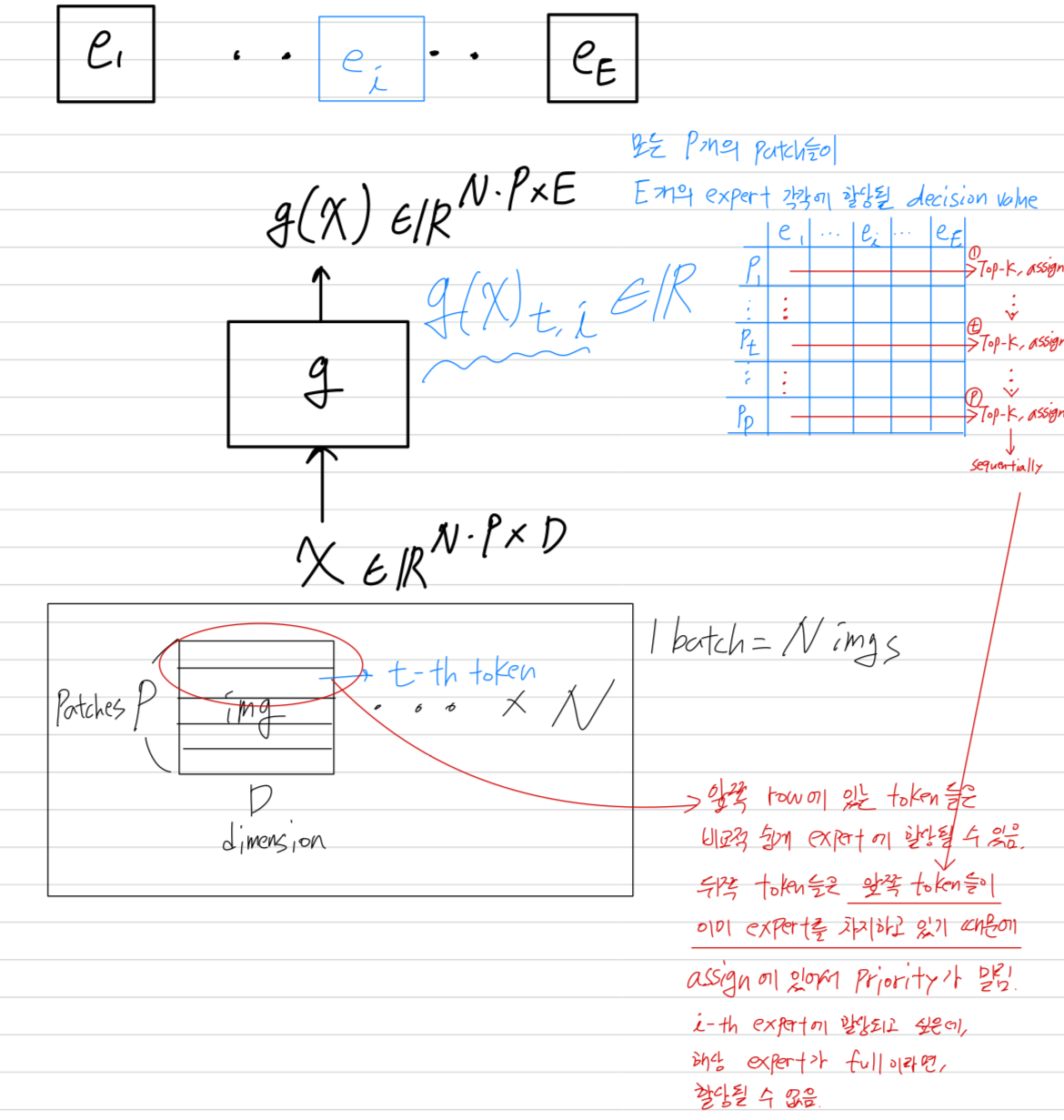
• Section 2의 notation을 사용하면, routing function $g$는 a batch of input $X \in \R^{N P \times D}$에 대해 row-wise로 적용된다.
  batch에는 $N$개의 image가 포함되며, 각 image는 $P$개의 token으로 구성된다.
  $X$의 각 row는 한 image의 특정 token의 $D$-dimensional representation을 나타낸다.
  

• 따라서 $g(X)_{t,i} \in \R$은 $t$-th token과 $i$-th expert에 대한 routing weight를 나타낸다.
  모든 routing algorithm에서, $i < j$일 경우, 모든 TOP-$i$ assignment는 TOP-$j$ assignment보다 priority를 갖는다.
  router는 먼저 모든 $i^{th}$ expert를 choice를 배정한 후, $j^{th}$ choice를 배정한다.
  [54]에서 사용된 the default-or vanilla-routing과 같이, TOP-$i$ position을 고려하면, routing은 다음과 같이 experts에게 tokens을 할당한다.
  router는 $g(X)$의 rows를 순차적으로 검사하여, expert's buffer가 not full할 때 해당 token을 TOP-$i$ expert에게 assign한다.
  결과적으로, token은 그에 해당하는 row의 rank에 따라 priority가 주어진다.
  batch 내 images는 randomly 정렬되지만, 각 image 내의 token은 pre-defined fixed order(미리 정의된 고정된 순서)를 따른다.
  

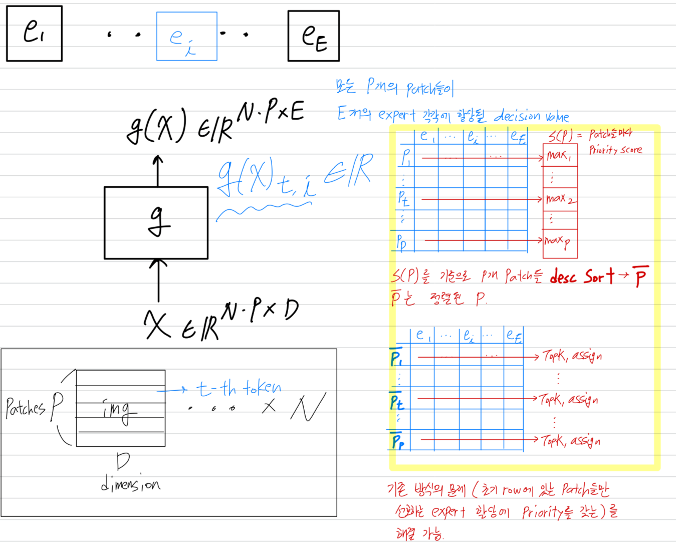
Batch Prioritized Routing (BPR)

• "most important" tokens을 우선시하기 위해, 각 token에 대한 priority score $s(x)$를 계산하고,
  이를 기반으로 $g(X)$를 sort하여 assign을 진행하는 방법을 제안한다.
  우리는 각 token을 그들의 maximum routing weight로 sort한다.
  공식적으로 $s(X)_t = \max_ig(X)_{t,i}$
  The sum of TOP-$k$ weights, 즉 $s(X)_t = \Sigma_ig(X)_{t,i}$도 동일한 성능을 보였다.
  이 두 가지 간단한 방법은 우리가 탐색한 다른 방법들보다 성능이 우수했다.
  

• 우리는 router outputs을 priority of allocation의 proxy(대리자)로 재사용했다.
  실험 결과, router output은 주로 tokens과 experts가 어떻게 짝지어질 수 있는지를 encoding하는데,
  final classification task에서 token의 "importance"를 나타내지 않지만, model의 predictive behaviour는 잘 유지했다.
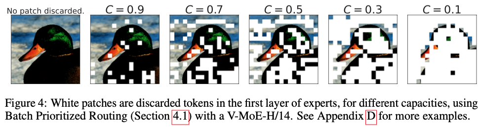
  Figure 4는 점차 작은 capacities에 대해 Batch Prioritized Routing을 통한 token prioritisation을 시각화한 것이다.
  batch $X$에 있는 모든 images에 있는 모든 tokens은 서로 경쟁하기 때문에, 서로 다른 image는 서로 다른 양의 computation을 받는다.
  

4.2 Skip tokens with low capacity C

• Batch Prioritized Routing은 어떤 tokens을 우선적으로 처리할지를 smartly selecting함으로써 buffer size를 줄이는 가능성을 열어준다.
  이는 overall sparse model의 computational cost에 극적인 영향을 미칠 수 있다.
  이제 $C << 1$ 조건에서section 2.4에서 정의된 기술 $C$를 기반으로 한 inference and training 결과를 discuss하겠다.

At inference time

• Prioritized routing은 model이 원래 어떻게 학습되었는지에 대해 독립적이다.
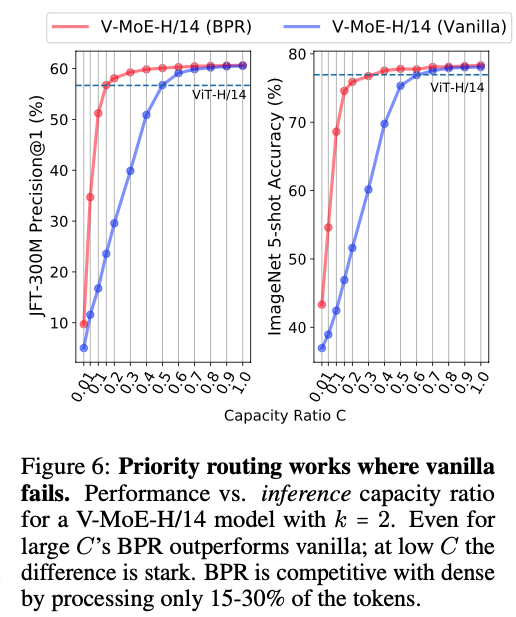
  Figure 6는 V-MoEe-H/14 model에서 BPR과 vanilla routing을 사용했을 때, inference 시 computing을 줄이는 효과를 보여준다.
  두 methods의 성능 차이는 특히 $C \le 0.5$에서 현저하게 나타난다.
  이 구간에서는 model이 실제로 token을 완전히 버리기 시작한다($k=2$).
  또한, BPR은 매우 낮은 capacity에서도 model이 dense model과 경쟁력을 유지할 수 있도록 한다.
  

• Figure 5에서 V-MoE-L/16과 V-MoE-H/14를 대상으로 보여주듯이,
  Batch Prioritized Routing과 low $C$ 값은 V-MoE가 inference 시 performance and FLOPs를 smoothly trade-off할 수 있게 하며, 이는 매우 독특한 model 특징이다.
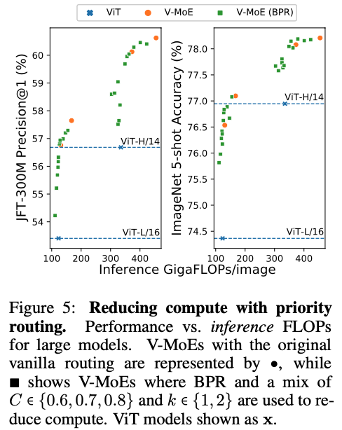  더 구체적으로, Table 10은 V-MoE model이 dense ViT-H 성능을 능가하면서도 FLOPs를 절반 이하로 줄이고, runtime을 60% 미만으로 줄일 수 있음을 보여준다.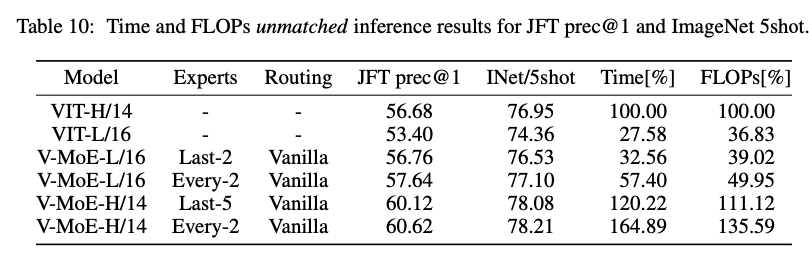반대로, FLOPs 비용을 동일하게 유지하면서 ImageNet/5-shot에서 one-ponit accuracy gain을,
  JFT에서는 3point에 가까운 Precision@1을 유지할 수있었다. (Table 11)
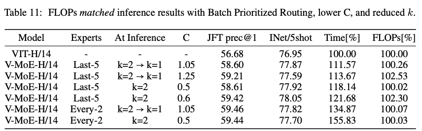  dense model은 일반적으로 동일한 FLOPs에 대해 V-MoE 구현에서 data transfer가 포함되므로 더 적은 runtime을 요구한다.

At training time

• Batch Prioritized Routing은 training 동안에도 활용될 수 있다.
  Appendix C에서는 max-weight routing을 사용하는 expert models이 dense performance를 유지하면서도 total training FLOPs의 약 20%를 절감할 수 있음을 보여준다.
  또한, 동일한 FLOP budget에서 vanilla routing을 훨씬 능가한다.