Abstract

• 우리는Network In Network(NIN)이라고 불리는 새로운 deep network structure를 제안한다.

• 우리는 receptive field에 대한 data를 더욱 abstract하는 complex structure로 micro neural networks를 만들었다.
  우리는 micro neural network를 multilayer perceptron로 예를 들어 설명한다.

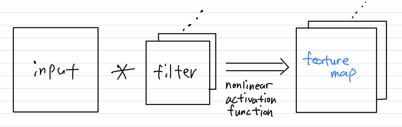
• The feature maps are obtained by sliding the micro networks over the input in a similar manner as CNN; they are then fed into the next layer.
  (The result outputs of convolution layer(not pooling layer) are called feature maps.)

• 우리는 NIN을 CIFAR-10, CIFAR-100, SVHN, MNIST dataset에 대해 state-of-the-art classification performance를 입증했다.

---

1. Introduction

• Convolutional Neural Networks(CNNs)은 convolutional layers와 pooling layers로 구성되어 있다.

  • Convolutional layer는 linear filter와 계산에 사용되는 receptive field의 inner product를 연산하고, every local portion에 nonlinear activation function을 적용한다.
    그 resulting outputs을 feature maps이라고 한다.
    

• The convolution filter in CNN is a generalized linear model(GLM) for the underlying data patch, and we argue that the level of abstraction is low with GLM.
  (convolution filter는 input에 대해 그저 linear한 계산만 하기 때문에 abstraction 능력이 적다.)

• GLM은 선형 계산을 하기 때문에 data가 linearly separable할 때, 좋은 abstraction 성능을 보일 수 있다.
  그래서 conventional CNN은 latent concepts에 대한 assumption을 linearly separable하게 만든다.
  하지만 data들은 보통 nonlinear한 공간에 있고, 이러한 공간을 capture하는 것은 일반적으로 input에 대한 nonlinear function이다.
  따라서 Replacing the GLM with a more potent nonlinear function approximator can enhance the abstraction ability of the local model.
그래서 In NIN, the GLM is replaced with a "micro network" structure which is a general nonlinear function approximator.
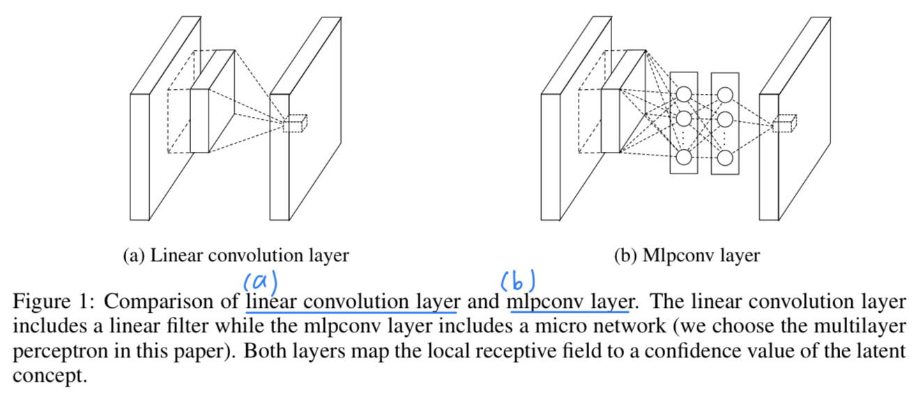  The resulting structure which we call an mlpconv layer is compared with CNN in Figure 1.
  The mlpconv maps the input local patch to the output feature vector with a multilayer-perceptron consisting of multiple fully connected layers with nonlinear activation functions.
  The MLP is shared among all local receptive fields.
  
  The overall structure of the NIN is the stacking of multiple mlpconv layers.
  It is called "Network In Network(NIN)" as we have micro networks (MLP)
  
  CNN에서 classification을 위해 traditional FC layers를 적용하는 대신,
  우리는global average pooling layer를 통한 category의 신뢰도로부터 마지막 mlpconv layer의 spaitial average를 output낸 다음,
  the resulting vector를 softmax layer에 입력하였다.
  (traditional CNN에서 FC layer는 두 사이의 관계에 대해서 black box 역할을 하기 때문에 객관적인 cost layer의 category level information이 어떻게 previous conv layer에서 지나갔는지 해석하기 어렵다.)?
  반면에, global average pooling은 feature map과 category 사이의 관계를 더욱 의미있고 해석할 수 있게 한다.
  
  게다가 FC layer는 parameter수가 매우 많아 overfitting이 따른다고 입증되었고 dropout regularization에 매우 의존한다고 밝혀졌지만,([4], [5])
  global average pooling은 그 자체로 regularizer 역할을 한다.

---

2. Convolutional Nerual Networks

• Classic convolution neuron networks consists of alternatively stacked convolutional layers and spatial pooling layers.
  The convolutional layers generate feature maps by linear convolutional filters followed by nonlinear activation functions(rectifier, sigmoid, tanh, etc.).
  Using the linear rectifier as an example, the feature map can be calculated as follows :
  
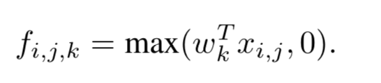
  $(i, j)$ is the pixel index in the feature map,
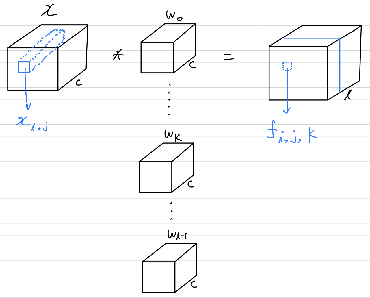
  $x_{i,j}$ stands for the input patch centered at location $(i,j)$
  , and $k$ is used to index the channels of the feature map.
  
  This linear convolution is sufficient for abstraction when the instances of the latent concepts are linearly separable.
  하지만 일반적으로 좋은 abstraction을 달성하는 representation은 input data에 대한 nonlinear function이다.
  conventional CNN에서는, 많은 filter를 이용함으로써 이를 보상할 수 있다.
  즉, 각각의 linear filter들은 can be learned to detect different variations of a same concept.
  하지만, single concept에 대한 너무 많은 filter는 다음 layer에 추가적인 부담을 준다.
  (next layer에서는 previous layer의 모든 분산의 combinations을 고려해야 한다.
  https://arxiv.org/pdf/1301.5088.pdf)
  
  It generates a higher level concept by combining the lower level concepts from the layer below.
  (CNN에서, 아래쪽 layer에서 lower level concept을 조합하여 higher level concept을 생성한다.)
  Therefore, higher level concept으로 combining하기 전에, 각 local patch를 abstraction하는 것이 더욱 이점이 있을 것이라고 주장한다.
  
  최근 maxout network 연구에서, maximum pooling을 함으로써 #feature maps이 줄어들었다.
  Maximization over linear function makes a piecewise linear approximator which is capable of approximating any convex functions.
  However maxout network imposes the prior that instances of a latent concept lie within a convex set in the input space, which does not necessarily hold.
  We seek to achieve this by introducing the novel "Network In Network" structure, in which a micro network is introduced with each convolutional layer to compute more abstract features for local patches.
  
  input에 대해 micro network를 sliding하는 것이 이미 몇차례 연구되었다.
  하지만 이전에 연구되었던 micro network들은 특정 task들에 특화된 것이었다.
  NIN은 more general perspective로 제안되었다.

---

3. Network In Network

• "Network in Network" structure에서 가장 중요한 key components :
  1. the MLP convolutional layer
  2. the global averaging pooling layer

3.1 MLP Convolution Layers

• 잠재 concept의 distribution에 대한 정보가 없을 때는 local patch들에 대한 feature extraction을 위한 universal function approximator를 사용하는게 바람직하다.
  Radial basis network와 multilayer perceptron은 universal function approximator로 잘 알려져있다.

• 우리는 두가지 이유로 multilayer perceptron를 선택했다.

  1. MLP is compatible(궁합이 잘 맞는다) with the structure of CNNs, which is trained using back-propagation.
  2. MLP can be a deep model itself, which is consistent with the spirit of feature re-use.[2]

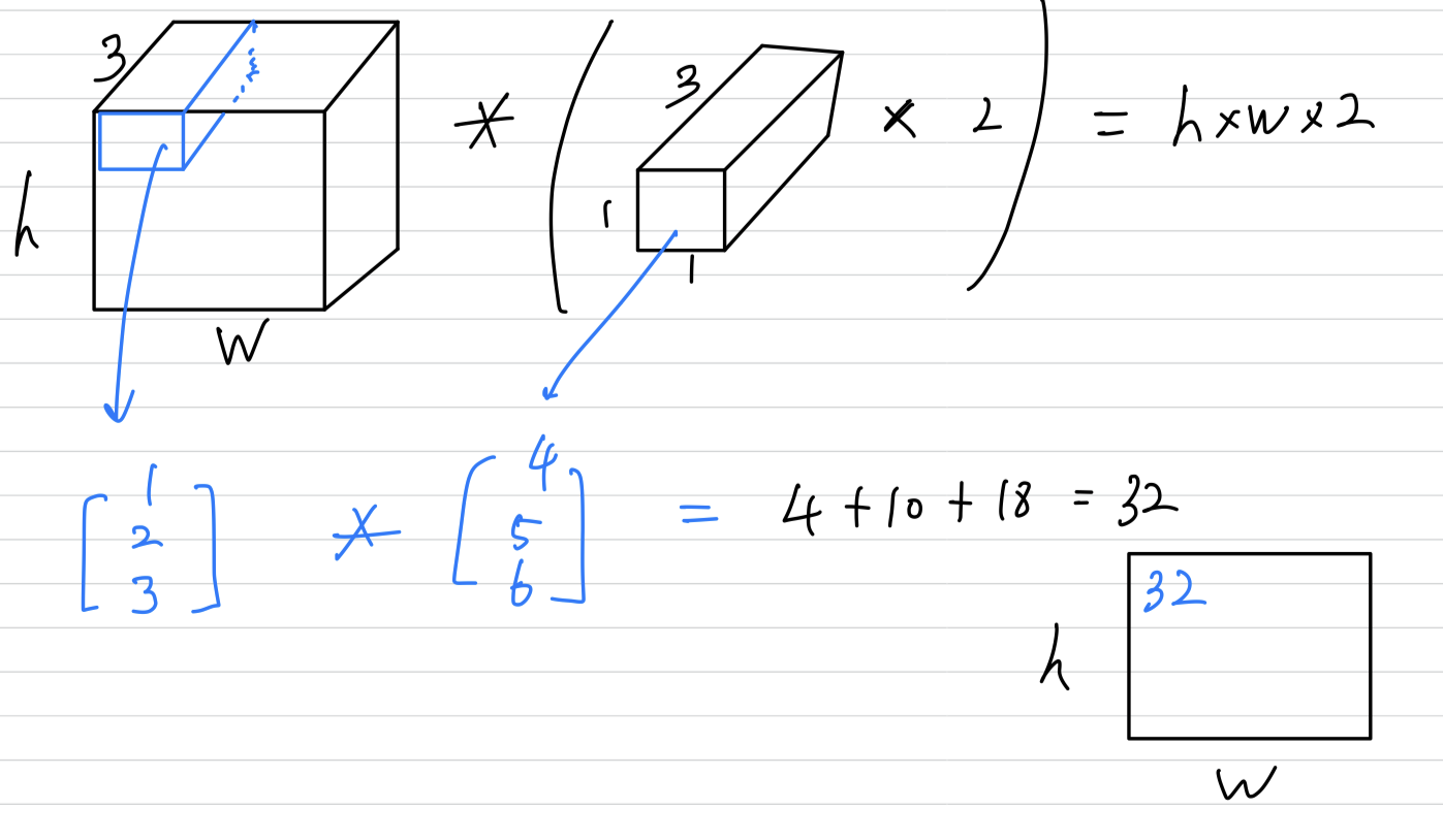
• The calculation performed by mlpconv layer is shown as follows :
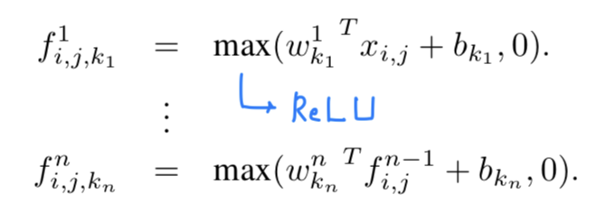  $n$ is the number of layers in the multilayer perceptron.
  ReLU is used as the activation function in the mlp.
  
  From cross channel(cross feature map) pooling point of view, Equation 2 is equivalent to cascaded cross channel parametic pooling on a normal convolution layer.
  This cascaded cross channel parameteric pooling structure allows complex and learnable interactions of cross channel information.
  The cross channel parametric pooling layer is also equivalent to a convolution layer with 1 x 1 convolution kernel.
  (Cross channel pooling : channel을 넘어 pooling을 하는 것.)
  This interpretation makes it straightforward to understand the structure of NIN.
  (➡️ 실제 mlpconv layer computation과 1 x 1 convolution은 다르다는 것을 암시할 수 있음. channel reduction 효과는 같지만 계산 방식이 다른데 저자가 이해를 돕기 위해 1 x 1 convolution과 같다고 말한 것 같음.)

3.2 Global Average Pooling

• For classification, the feature maps of the last conv layer are vectorized and fed into FC layers followed by a softmax logistic regression layer.
  However the FC layers are prone to overfitting, thus hampering generalization ability of the overall network.
  
  In this paper, we propose another strategy called Global Average Pooling(GAP) to replace the traditional FC layers in CNN.
  We take the average of each feature map, and the resulting vector is fed directly into the softmax layer.
  
  One advantage of GAP over the FC layers is that feature map들과 category들 사이의 correspondence(상응, 대응)을 강화함으로써 convolution structure에 더욱 적합하다. (CAM : Class Activation Map)
  Another advantage is that there is no parameter to optimize in the global average pooling thus overfitting is avoided at this layer.

3.3 Network In Network Structure

• The overall structure of NIN is a stack of mlpconv layers, on top of which lie the GAP and the objective cost layer.
  Within each mlpconv layer, there is a three-layer perceptron.

4. Experiments

4.1 Overview

• We evaluate NIN on 4 benchmark datasets : CIFAR-10, CIFAR-100, SVHN and MNIST.

• The network used for the datasets all consist of 3 stacked mlpconv layers, and the mlpconv layers in the experiments are followed by a spatial max pooling layer which downsamples the input image by a factor of two.

• dropout is applied on the outputs of all but the last mlpconv layer.

• All the networks used in the experiment section use global average pooling instead of FC layers at the top of the network.

• Another regularizer applied is weight decay(0.0005) as used by Krizhevsky et al. [4]

• We implement our network on the super fast cuda-convnet code developed by Alex Krizhevsky [4].

• Preprocessing of the datasets, splitting of training and validation sets all follow Goodfellow et al. [8]

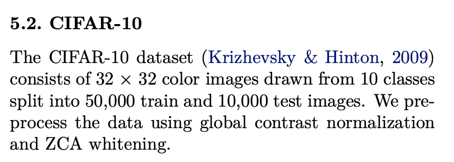
  • CIFAR-10 :
    ➡️ 50,000 train images
    ➡️ 10,000 test images
    ➡️ preprocess the data using global contrast normalization and ZCA whitening.
    
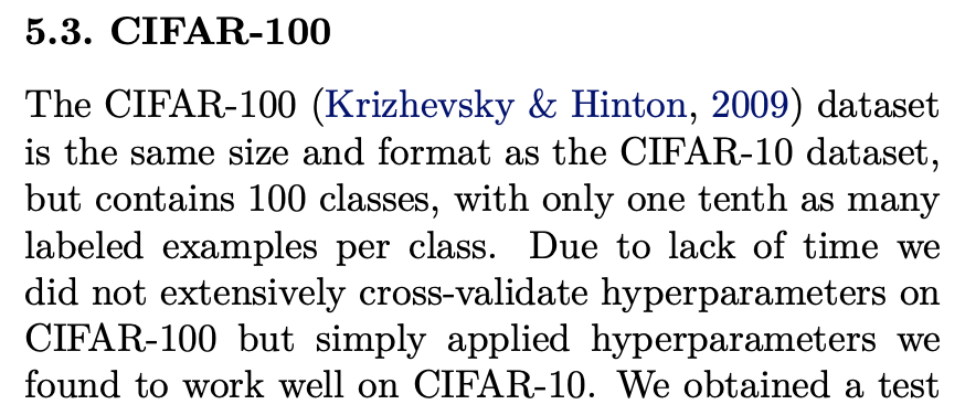
  • CIFAR-100 :
    ➡️ CIFAR-10 dataset과 똑같음. (100 class라는 것만 다름.)
    
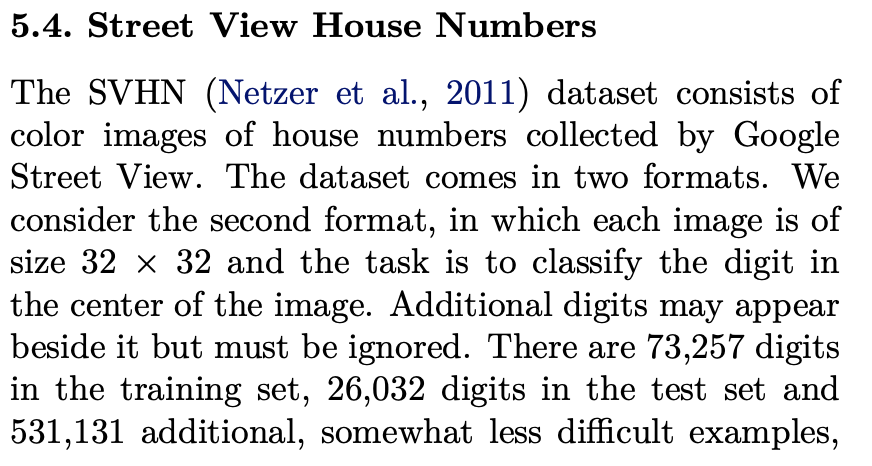
  • SVHN(Street View House Numbers) :
    ➡️ SVHN dataset은 color image로 구성되어 있고, 2가지 format이 있다.
    ➡️ 우리는 두번째 format을 고려한다. (32 x 32 size의 image 중앙의 숫자를 분류하는 작업)
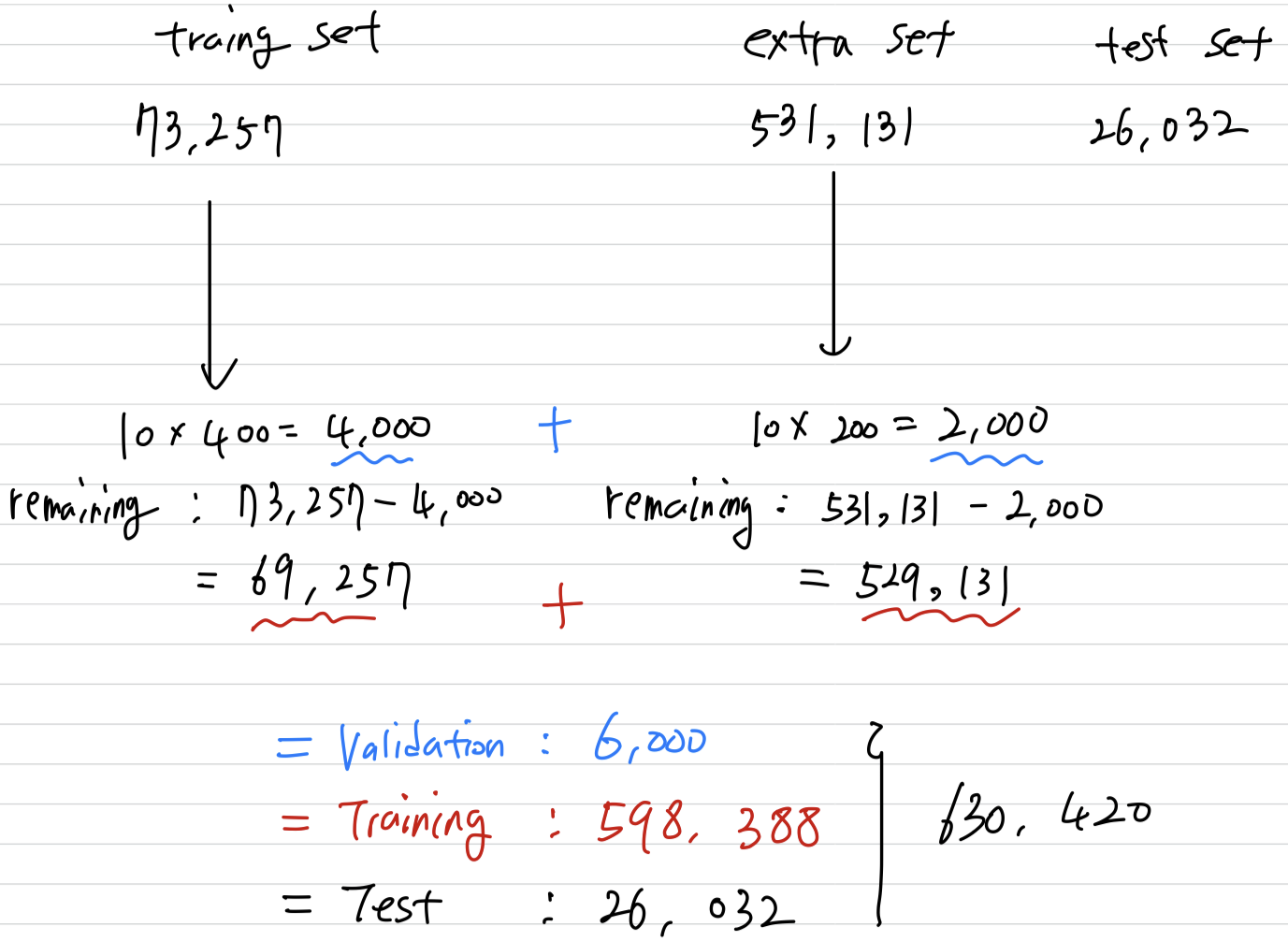
    ➡️ 73,257 training set
    ➡️ 26,032 test set
    ➡️ test set으로 사용하기 어려운 extra set에 531,131 sample가 있는데,
    Sermanet et al.(2012b)에 따르면 training set에서 class 당 400samples와 extra set에서 class 당 200samples 를 validation set으로 사용했다.
    나머지 train과 extra sets sample들은 training을 위해 사용되었다.
    
  • MNIST :
    ➡️ 60,000 training images
    ➡️ 10,000 testing image

• The network is trained using mini-batches of size $128$.

• training set에 대한 accuracy 향상이 멈출 때까지 initial weight and learning rate를 사용.
  accuracy 향상이 멈추면 learning rate 10씩 나눠줌.
  이 과정을 initial value의 1%가 될 때까지 진행 (accuracy 향상 멈추는게 3번째 되면, 학습 종료한다는 얘기인듯 = 10으로 나눠주는 걸 2번만 했다는 얘기인듯)

4.2 CIFAR-10

• The CIFAR-10 is composed of 10 classes of natural images with $50,000$ training images, and $10,000$ testing images.
  We use the last $10,000$ images of the training set as validation data.

• Each image is an RGB image of size 32 x 32.

• For this dataset, we apply the same global contrast normalization and ZCA whitening as was used by Goodfellow et al. in the maxout network.

• maxout network와 일치하도록 각 mlpconv layer의 feature map 수를 똑같이 하였다.
  Two hyper-parameter(local receptive field size, the weight decay)는 validation set을 이용하여 tuning되었다.

• hyper-parameter가 고정되어지고 우리는 network를 re-train시켰다.

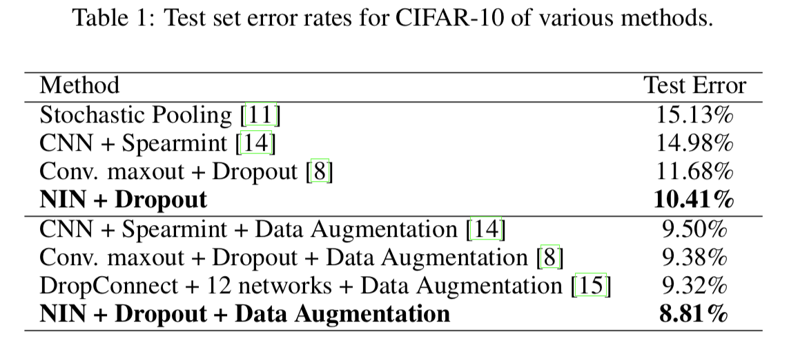
• 우리는 state-of-the-art보다 1% 향상된 10.41%의 test error를 얻었다.
  

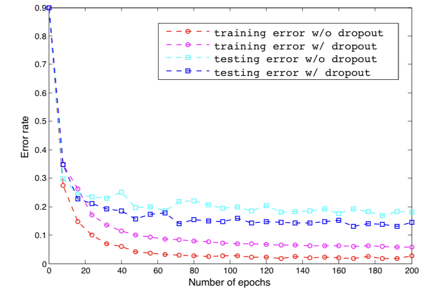
• NIN의 mlpconv layer 사이에 dropout을 사용하는 것이 model의 generalization 능력을 향상시키는 데에 효과가 있음을 밝혀냈다.
  As in shown in Figure 3, introducing dropout layers in between the mlpconv layers reduced the test error by more than 20%.
  그러므로 이 논문에서 사용된 모든 model들은 mlpconv layer들 사이에 dropout이 적용되었다.
  

• 추가적으로 translation and horizontal flipping augmentation을 사용했더니 test error of 8.81% 달성.

4.3 CIFAR-100

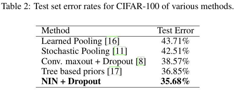
• The CIFAR-100 is the same in size and format as the CIFAR-10 dataset, but it contains 100 classes.
  Thus the number of images in each class is only one tenth of the CIFAR-10 dataset.

• The only difference is that the last mlpconv layer outputs 100 feature maps.
  

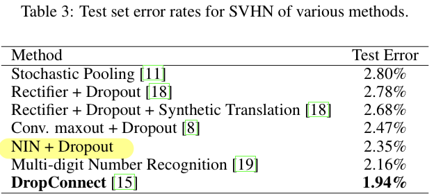
4.4 Street View House Numbers

• SVHN dataset은 color image로 구성되어 있고, 2가지 format이 있다.
  우리는 두번째 format을 고려한다. (32 x 32 size의 image 중앙의 숫자를 분류하는 작업)
  ➡️ 73,257 training set
  ➡️ 26,032 test set
  ➡️ test set으로 사용하기 어려운 extra set에 531,131 sample가 있는데,
  Sermanet et al.(2012b)에 따르면 training set에서 class 당 400samples와 extra set에서 class 당 200samples 를 validation set으로 사용했다.
  나머지 train과 extra sets sample들은 training을 위해 사용되었다.
  

• The training set and the extra set are used for training.
  The validation set is only used a guidance for hyper-parameter selection, but never used for training the model.

• Preprocessing of the dataset again follows Goodfellow et al. ,which was a local contrast normalization.

• The structure and parameters consist of three mlpconv layers followed by GAP.

• For this dataset, we obtain test error rate of 2.35%.
  

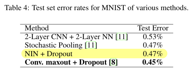
4.5 MNIST

• The MNIST dataset consists of hand written digits 0-9 which are 28x28 in size.
  There are 60,000 training images and 10,000 testing images in total.

• For this dataset, the same network structure as used for CIFAR-10 is adopted.
  But the nmber of feature maps generated from each mlpconv layer are reduced.
  Because MNIST is the simpler dataset compared with CIFAR-10 ; fewer parameters are needed.

• We test our method on this dataset without data augmentation.
  

4.6 Global Average Pooling as a Regularizer

• Global average pooling layer is similar to the FC layer in that they both perform linear transformations of the vectorized feature maps.

• The difference lies in the transformation matrix.
  For GAP, the transformation matrix is prefixed and it is non-zero only on block diagonal elements which share the same value.
  FC layers can have dense transformation matrices and the values are subject to back-propagation optimization.
  (FC layer는 backprop으로 optimization해야 하는 대상이고, feature map과 FC layer 사이에 매우 많은 Parameter가 존재하니까 overfitting의 위험이 있다)

• To study the regularization effect of global average pooling, we replace the global average pooling layer with a FC layer, while other parts of the model remain the same.
  GAP를 사용한 model과 FC layer 전에 dropout 없이 사용한 model을 CIFAR-10 dataset에 대하여 비교해봤다.
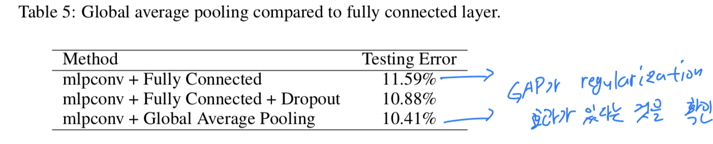  This is expected as the FC layer overfits to the training data if no regularizer is applied.
  Global average pooling has achieved the lowest testing error(10.41%) among the three.

4.7 Visualization fo NIN

• We explicitly enforce feature maps in the last mlpconv layer of NIN to be confidence maps of the categories by means of global average pooling, which is possible only with stronger local receptive field modeling,, e.g. mlpconv in NIN.

• To understand how much this purpose is accomplished, we extract and directly visualize the feature maps from the last mlpconv layer of the trained model for CIFAR-10.

• Figure 4 shows some examplar images and their corresponding feature maps for each of the ten categories selected from CIFAR-10 test set.
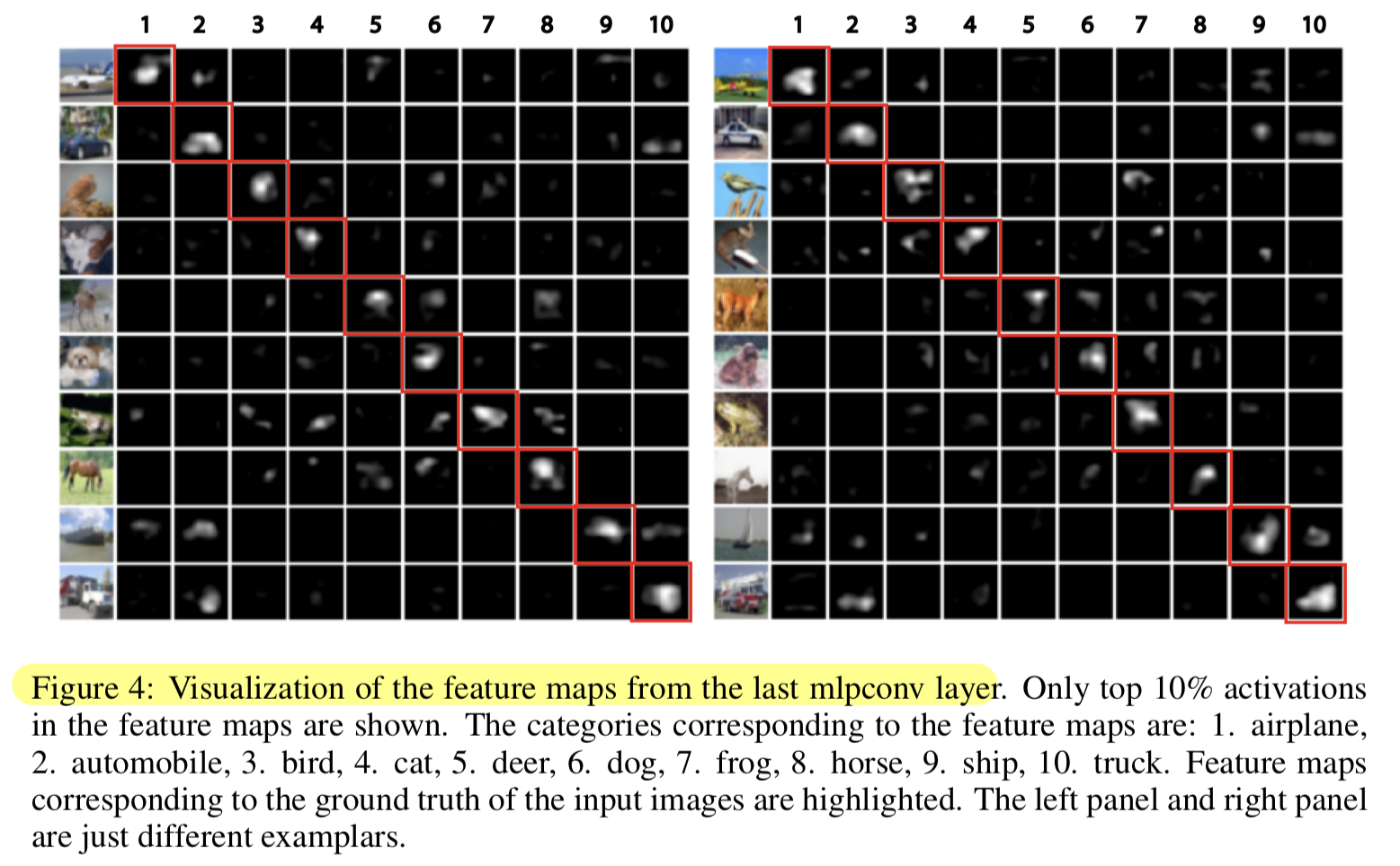  It can be observed that the strongest activations appear roughly at the same region of the object in the original image.
  The visualization again demonstrates the effectiveness of NIN.
  It is achieved via a stronger local receptive field modeling using mlpconv layers.
  The global average pooling then enforces the learning of category level feature maps.

---

5. Conclusions

• 우리는 classification task를 위한 "Network In Network"(NIN)이라고 불리는 deep network를 제안했다.

• NIN은 input에 대해 MLP로 convolution하는 mlpconv layer와 FC layer를 대신한 Global Average Pooling layer로 구성된다.

• Mlpconv layers는 local patch를 더 잘 되게 하고, GAP는 overfitting을 막는 regularizer로 역할ㄹ을 한다.
  이 두 components로 우리는 CIFAR-10, 100, SVHN dataset에 대해 state-of-the-art performance를 보였다.

• Through visualization of the feature maps,
  we demonstrated that feature maps from the last mlpconv layer of NIN were confidence maps of the categories, and this motivates the possibility of performing object detection via NIN.

---

내 생각, 궁금한 점

• Introduction만 읽은 후, 좋은 아이디어같긴 한데 parameter가 너무 많아서 비효율적일 것 같다.
  그냥 nonlinear activation function으로만 nonlinear 연산을 하는 것이 learning의 효과는 더 적을지 몰라도 parameter수를 매우 많이 아낄 수 있을 것 같다.
  (직접 NIN과 normal model을 train시켜본 후, accuracy 차이와 #params 차이를 확인해보면 좋을 것 같다.)

• universal function approximator로 Radial basis network 대신에 mlp를 사용한 이유를 정확히 모르겠다..

  1. Radial basis network란?
  2. Radial basis network와 CNN은 not compatible한가? 왜 그런가?
  3. MLP 대신 Radial basis network를 적용하여 NIN을 만들어본다면?

• mlpconv layer의 computation은 1 x 1 convolution과 다르다고 생각했었는데,
  "The cross channel parametric pooling layer is also equivalent to a convolution layer with 1x1 convolution kernel"
  위 문장 때문에 mlpconv layer computation과 1 x 1 convolution에 대해서 이해가 안되기 시작했다.
  우선 나의 결론은 mlpconv layer computation과 1 x 1 convolution은 전혀 다른 연산이다.
  결과적으로 나오는 feature map의 channel이 축소된다는 점은 공통사항이지만 연산 방법이 아예 다른 거라고 이해했다.
  우선 내가 아는 1 x 1 convolution은 다음과 같다.
  
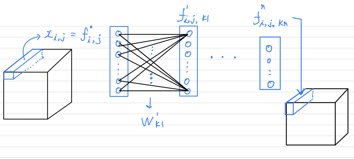
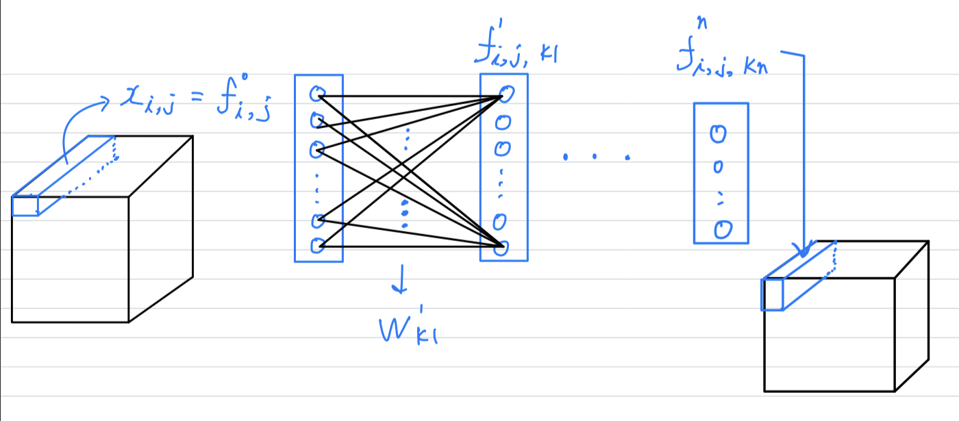
  그리고 내가 이해한 mlpconv layer는 다음과 같다.
  (나의 생각) :
  1 x 1 convolution과 같은 점은 오로지 input과 ouput volume의 크기(channel reduction)이다.
  다른 점은 연산 과정에서 1 x 1 convolution은 convolution 계산을 하였고,
  mlpconv layer에서는 Multi Layer Perceptron들이 있어서 convolution 연산이 아니라 fully connected layer 계산을 하였다. 그래서 Parameter가 훨씬 더 많을 것이다.
  
  또한 저자가 "This interpretation makes it straightforawrd to understand the structure of NIN." 라고 썼는데,
  1 x 1 convolution의 개념이 없었을 때라 독자의 이해를 돕기 위해 "1 x 1 convolution과 같은 연산이다"라고 했던 것이지 현재 우리가 알고 있는 1 x 1 convolution의 계산과는 다른 것이라고 생각한다.
  (channel reduction 효과는 같지만 계산 방식이 다른데 저자가 이해를 돕기 위해 1 x 1 convolution과 같다고 말한 것 같음.)

  (궁금증) : 그럼 만약 NIN에서 사용한 mlpconv layer(1 x 1 convolution으로 비유한)의 computation을 실제 1 x 1 convolution으로 바꾸면 어떻게 될까?
  정확도가 더 높아질까? 낮아질까?

• 저자가 NIN의 overall structure라고 첨부한 Figure 2이다.
  
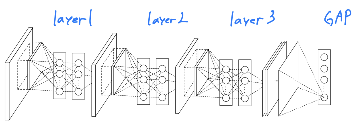
  위 그림 때문에 이해하기 훨씬 어려웠다.
  내가 글을 읽으며 이해한 하나의 mlpconv layer는 다음과 같다.
  (나의 생각) : 저자가 첨부한 그림으로는 cascaded cross channel pooling 방식이 어떻게 적용되었다는 건지 정확하게 설명된 것 같지 않고, 오히려 이해를 방해하는 그림인 것 같다.

• 4.6에서 CIFAR-10 말고 다른 dataset으로 해봐도 똑같이 GAP가 잘 될까?
  그리고 Dropout을 적용해봐서 더 잘 되면 parameter가 많더라도 FC+dropout을 사용하는 것이 더 낫지 않을까?

• 4.7에서 "The global average pooling then enforces the learning of category level feature maps." 부분에서 GAP말고 FC layer + dropout을 사용했을 때 마지막 mlpconv layer의 feature map을 10으로 하고 visualization해도 저렇게 나오지 않을까?
  = GAP가 feature map의 category 능력을 학습하는 것을 강화하는 것은 모르겠지만,
  FC layer + dropout도 마찬가지 아닐까?

---

Seminar - discussion

• Representation이란?
  Input에서 변한 또 다른 결과물을 representation이라고 한다.
  원래 갖고 있던 data의 "표현"이 다른 "표현"으로 바뀌는 것임.
  parameter를 바꾸면 중간 layer에서의 representation들이 계속해서 바뀐다.
  그래서 Deep Learning을 Deep Representation Learning이라고도 한다.

• Global Average Pooling의 가장 큰 장점으로는
  input size가 달라져도 영향을 받지 않는다는 것이다.
  기존의 FC layer로 classification할 때보다 model이 더욱 유동적이다.
  
  또한 feature map의 중요성 정보라던지 그런 것들이 유지될 수 있다.
  FC는 공간적 정보를 모두 섞어버려서 좋지 않을 수 있다. (추후 CAM 논문)

• Network in Network structure의 가장 큰 의의로는
  module의 개념이 등장했다는 것이다.
  이전의 AlexNet, VGGNet은 Layerdml dusthrdldjTekaus
  NIN은 Layer를 반복시키는 것도 맞지만 layer 안에 또 다른 layer들이 있기 때문에
  module, block의 개념을 등장시켰다.