[Vision Paper Review] - Attention Is All You Need

Vision Transformer 관련된 논문 리뷰의 가장 첫 번째 포스트로는 NLP(자연어처리)에서 가장 큰 영향을 주고 있고, Vision에서도 쓰이고 있는 Transformer를 가장 먼저 리뷰해보겠습니다. 논문과 공식 Github Code는 아래 링크를 참고해주세요.

✅Attention is All You Need
✅Official Tensorflow Code - Github

Abstract

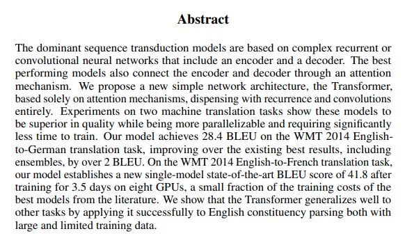Fig 1. Abstract

Abstract에서는
1. "The dominant sequence transduction models are based on complex reccurent or convolutional neural networks that include encoder and decoder"
2. "~ based solely on attention mechanisms , dispending with recurrence and convolutions entirely."

이 두 문장으로 본 연구의 전반적인 목적과 성과를 설명하고 있습니다. Transformer 이전의 모델들은 RNN과 CNN을 사용하는 것이 주를 이루었고, 가장 성능이 좋은 모델 또한, Attention mechanisms에 Encoder와 Decoder를 연결한 구조였습니다. 이와 달리, Transformer는 오직 attention mechanisms을 사용하며, RNN과 CNN을 포함하고 있지 않습니다. 따라서 이를 통해 본 논문의 제목인 "Attention is All You Need" 를 이해할 수 있습니다. 이 구조를 통해서 Engligh-to-German, English-to-French Translation task에서 좋은 성능을 보였다고 정리하고 있습니다.

Introduction

RNN, LSTM(Long Short-Term Memory), gated RNN이 기존에 제기된 Sequence modeling과 Transduction problem에 SOTA를 달성했습니다.
본 Paper에서는 이런 Recurrent model의 문제점을 제시했는데,

"This inherently sequential nature precludes parallelization within training examples, which becomes critical at longer sequence lengths,"

즉, Recurrent model은 parallelization이 불가능하여 longer sequetial length에서 치명적인 단점이 있습니다. 비록 최근의 연구결과(그 당시에)들이 computational efficiency와 model performance를 향상시켰지만, 근본적인 문제점은 여전히 남아있습니다.

Attention mechanisms은 다양한 분야에서 접목되서 사용되고 있었으나, 기존에 사용되고 있는 Recurrent model에 conjugated된 형태로만 사용되고 있었습니다. Attention mechanisms의 장점은 input과 output sequence의 distance에 상관없다는 것 입니다.

" ~ allowing modeling of dependencies without regard of their distance in the input or output sequences"
" ~ however, such attention mechanisms are used in cojunction with a recurrent network."

본 연구는 Transformer를 제시하는데,

"relying entirely on an attention mechanism to draw global dependencies between input and output."

기존에 제기되었던 parallelization을 해결할 수 있어서 더 짧은 시간에 좋은 성능을 보였다고 합니다.

Background

Sequential Computation을 줄이는 것은 Extended Neural GPU, ByteNet, ConvS2S에서도 제시되었지만,

• all of which use CNN as basic building block
• Computing hidden representations in parallel for all input and output positions

의 방식을 사용하여 more difficult to learn dependencies between distance position 이란 문제점이 있습니다.

또한 Background에서 Self-Attention(Intra-Attention), End-to-End Memory Network에 대해서도 간략히 서술해두었습니다. 아래 Fig 2.를 참고해주세요.

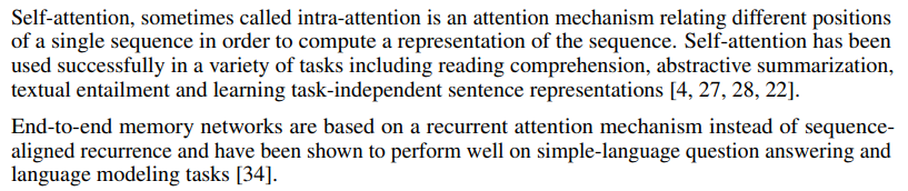Fig 2. Background

이런 Background를 기반으로 본 논문에서는 Transformer를 아래와 같이 소개하고 있습니다.

" the first transduction model relying entirely on self-attention to compute representations of its input and output without using sequence-aligned RNNs or convolutions"

Model Architecture

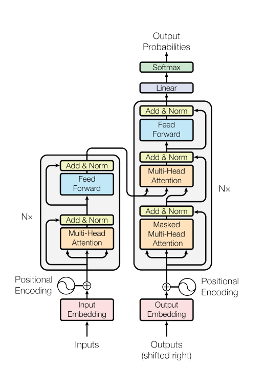Fig 3. Transformer Model Architecture

Encoder and Decoder Stacks

Encoder

Encoder의 특징은 아래와 같습니다.

• Encoder is composed of a stack of N = 6 (본 논문에서 6으로 설정)
• Each layer has two sub-layers
  (Multi-Head Self-Attention & Position wise fully connected feed-forward network)
• Employ a residual connection followed by layer normalization
• Output of each sub-layer
  $LayerNorm( x + SubLayer(x))$
• produce outputs of dimension
  $d_{model} = 512$

Decoder

Decoder의 특징은 아래와 같습니다.

• Decoder is composed of a stack of N = 6 (Encoder와 동일)
• The decoder insert a third sub-layer, which performs multi-head attention over the output of the encoder stack.
• 그 외 특성은 Encoder와 유사

Attention

아래는 Attention function에 대한 간략한 설명입니다.

"An attention function can be described as mapping a query and a set of key-value pairs to an output, where the query, keys, values, and output are all vectors. The output is computed as a weighted sum of the values, ~ "

Attention Function에 대한 이론적인 부분은 ✔ 딥러닝을 이용한 자연어처리 입문 ✔에서 보다 상세히 소개되어 있으니, 참고하면 도움이 될 것 같습니다.

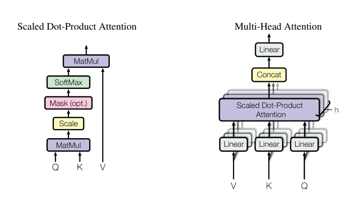Fig 4. Scaled Dot-Product Attention(L) & Multi-Head Attention consists of several attention layers running in parallel(R)

Scaled Dot-Product Attention

Fig 4(L)을 참고하여 특징을 정리하면,

• The input consists of queries and keys of dimension $d_k$, and values of dimension $d_v$
• compute the dot prodict of the query with all ppeys, divide each by $\sqrt{d_k}$
• apply softmax function to obtain the weights on the values
  $Attention(Q, K, V) = softmax(\frac{QK^{T}}{\sqrt{d_k}})V$

가장 많이 사용되는 Attention function 중 대표적인 두 가지는

1. Additive Attention : computes the compatibility function using a feed-forward network with a single hidden layer.
2. Dot-Product(Multiplicative) Attention : identical to our algorithm, except for the scaling factor of $\frac{1}{\sqrt{d_k}}$

이 있습니다. 두 가지 함수는 이론적인 복잡도 측면에서는 유사하지만 Dot-Product Attention이 더 빠르고, 공간적으로 효율적입니다.

" While the two are similar in theoretical complexity, dot-product attention is much faster and more space-efficient in practice, since it can be implemented using highly optimized matrix multiplication code"

작은 $d_k$ 값에서는 두 메커니즘이 비슷한 성능을 보이지만, additive attention이 $d_k$값이 증가할 수록 성능이 좋다고 합니다. 본 연구에서는 큰 값을 사용하기 때문에 dot-product의 gradient vanishing problem이 일어날 수 있어, dot-product를 $\frac{1}{\sqrt{d_k}}$로 scaling 해주었습니다.

" While for small values of dk the two mechanisms perform similarly, additive attention outperforms dot product attention without scaling for larger values of $d_k$. We suspect that for large values of $d_k$, the dot products grow large in magnitude, pushing the softmax function into regions where it has extremely small gradients. To counteract this effect, we scale the dot products by $\frac{1}{\sqrt{d_k}}$ "

Multi-Head Attention

Fig 4(R)을 참고하며, $d_{model}$ - demensional keys, values, queries를 사용한 single attention function 보다 queries, keys, and values를 서로 다르고, 학습된 linear projection을 $d_k, d_k, d_v$ 차원에 수행하는 것이 더 효과적인 것을 발견했습니다. 이렇게 projected 된 version의 Q, K, V는 병렬로 attention function을 거치게 되고, $d_v-demensional$ output value를 얻게 됩니다. 이는 Concatenated되고 다시 projected 되어 최종값을 도출합니다.

"Multi-head attention allows the model to jointly attend to information from different representation subspaces at different positions. With a single attention head, averaging inhibits this."

사용된 파라미터들을 정리하면 아래와 같습니다.

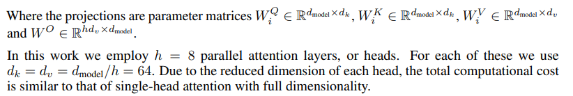Fig 5. Parameters

Applications of Attention in our Model

Transformer는 Multi-head Attention을 3가지 다른 방법으로 사용했습니다.

Encoder-Decoder Attention

• Queries come from the previous decoder layer
• Memory keys and values come from the output of the encoder
  ➡ This allows every position in the decoder to attend over all positions in the input sequence

Encoder

• Encoder contains self-attention layers
• In a self-attention layer all of the keys, values and queries come from the same place
  ➡ Each position in the encoder can attend to all positions in the previous layer of the encoder

Decoder

➡ self-attention layers in the decoder allow each position in the decoder to attend to all positions in the decoder up to and including that position.

• need to prevent leftward information flow in the decoder to preserve the auto-regressive property
• implement thisinside of scaled dot-product attention by masking out (setting to −∞) all values in the input of the softmax which correspond to illegal connections

Position-wise Feed-Forward Networks

본 모델의 Encoder와 Decoder는 모두 FFN을 가지고 있습니다. 이 FFN은 각 위치에 개별적이고 분리되어서 적용되며, ReLU 함수가 중간에 위치한 두 개의 선형 변환으로 이루어져 있습니다.

each of the layers in our encoder and decoder contains a fully connected feed-forward network, which is applied to each position separately and identically. This consists of two linear transformations with a ReLU activation in between.

FFN의 수식은 다음과 같습니다.

각 선형 변환은 다른 위치에 있어도 동일하지만, layer 마다 다른 parameter를 사용합니다.

Embeding and Softmax

• Sequence transduction model과 유사하게, 학습된 embedding을 input token과 output token을 $d_{model}$ dimension 상의 벡터로 변환하기 위해 사용
• usual learned linear transformation과 softmax function을 decoder output을 predicted next-token prob로 변환하기 위해 사용
  -> same weight matrix가 two embedding layer와 pre-softmax linear transformation에서 사용됨
• Multiply $\sqrt{d_{model}}$ to those weights

Positional Encoding

Transformer는 어떠한 recurrance와 convolution을 사용하지 않기 때문에, 본 연구에서는 sequence를 사용하기 위해 sequence의 token들에 대한 상대적, 그리고 절대적인 위치 정보를 삽입해줘야합니다.

" Since our model contains no recurrence and no convolution, in order for the model to make use of the order of the sequence, we must inject some information about the relative or absolute position of the tokens in the sequence. "

따라서 본 연구에서는 positional embedding을 encoder와 decoder stack의 아래의 input embedding에 삽입하였습니다. Positional Encoding은 Embedding과 마찬가지로 $d_{model}$의 차원을 가져 덧셈 연산(summation)이 가능하고, 다양한 함수를 사용할 수 있지만, 본 연구에서는 sine, cosine 함수를 서로 다른 주파수 영역에서 사용했습니다. 수식은 아래와 같습니다. 본 함수를 사용한 이유는 주기성으로 k번째 식도 표현할 수 있기 때문입니다.( 이렇게 보면 삼각함수가 참 중요한 것 같습니다. 주기성이라는 특성 하나만으로도요.)

연구진은 학습된 positional embedding에 대해 실험을 진행했고, 두 가지 결과가 비슷하게 도출되었습니다. 이를 기반으로 sine 함수를 사용했는데,

"it may allow the model to extrapolate to sequence lengths longer than the ones encountered during training."

의 사유, 즉 model이 더 긴 길이의 sequence를 유추할 수 있게 해주기 때문입니다.

Why Self-Attention

본 문단에서는 self-attention과 기존에 사용되던 (state-of-the-art) RNN 등과의 비교가 주를 이룹니다. 첫 번째로 비교한 것은 전체적인 연산의 복잡도이며, 그 결과는 논문의 Table.1 (본 정리본의 Fig .6)에 나와있습니다. 두 번째는, parallel 하게 연결 할 수 있는 연산의 총 수이며, 마지막 세번째는 네트워크 상에서 path 간의 long-range dependencies 입니다.

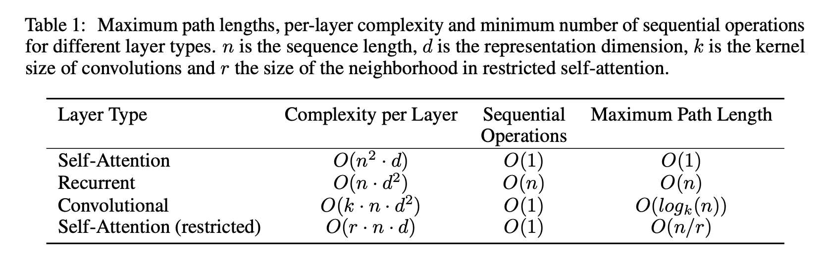Fig 6. Table 1 in Paper

• Self-Attention Layer는 모든 Position을 상수인 시간에만 연결
• Recurrent Layer는 $O(n)$의 시간 복잡도를 가짐
• Layer가 $n(=sequence \; length) < d(representation \; dimensionality)$ 일 때 self-attention layer가 더 효율적임
• very-long sequence에 대해서는 self-attention은 neighborhood size를 $r$로 제한할 수 있고, 이는 max path-length를 $O(n/r)$로 증가시킬 수 있음
• $k<n$ 인 kernel width 의 single convolutional layer는 input 과 output의 모든 쌍을 연결하지 않음
  ➡ contiguous kernel의 경우 $O(n/k)$의 stack이 필요
  ➡ dilated convolution의 경우 $O(log_k(n))$이 필요
• Convolution layer는 일반적으로 recurrent layer보다 더 큰 비용이 요구
  ➡ Separable Convolution의 경우 복잡도를 $O(k \cdot n \cdot d+n \cdot d^2)$ 까지 줄일 수 있음
• $k = n$ 의 경우, transformer 와 같이 self-attention layer와 point-wise feed forward layer의 조합과 복잡도가 같음

Training

Training에 대한 기본 세팅 등은 논문 상에 소개된 부분으로 이미지로 대체합니다. Fig 7 ~ 8을 참고 해주세요.

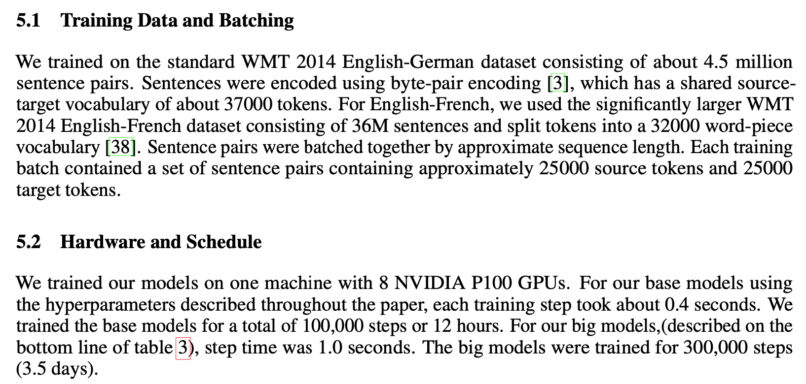Fig 7. Training Data and Batching & Hardware and Schedule

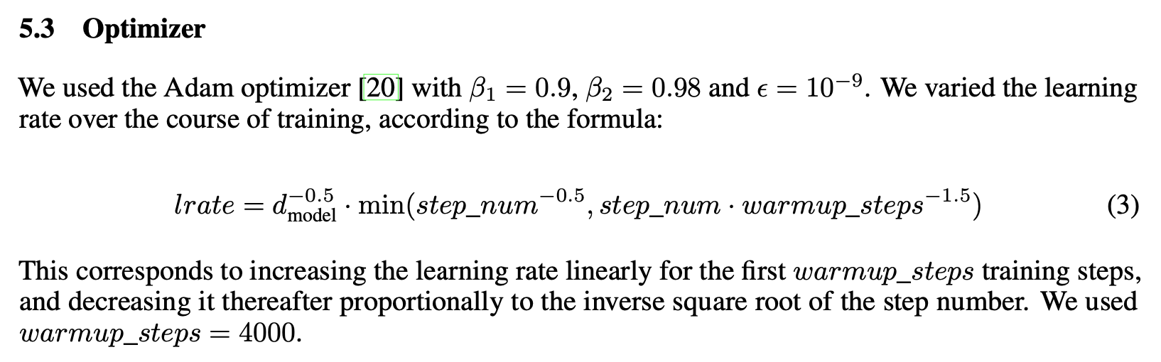Fig 8. Optimizer

본 연구에서는 ADAM을 Optimizer로 사용했습니다.

Regularization

본 연구에서는 세 가지 Regulaization을 사용했는데요.

1. 각 sub-Layer의 Output이 다음 sub-layer에 input에 더해지고 normalization 되기 전에 Residual Dropout 적용
2. Encoder & Decoder stack의 positional embedding과 sums of embedding에 dropout 적용
3. 학습 중에 labeling smoothing 적용

Results

Machine Translation

Model Variations

English Constituency Parsing

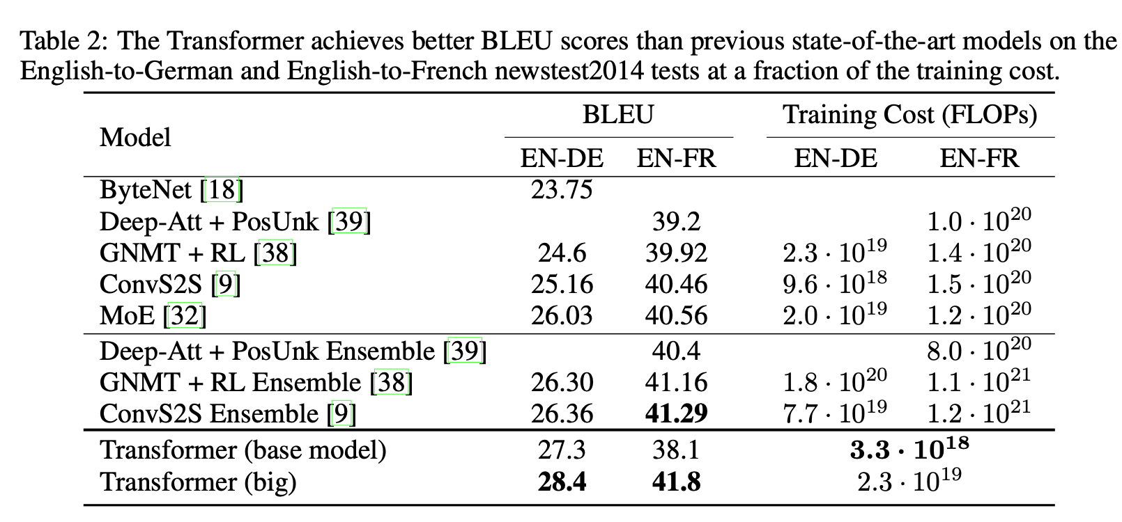Fig 9. Table. 2

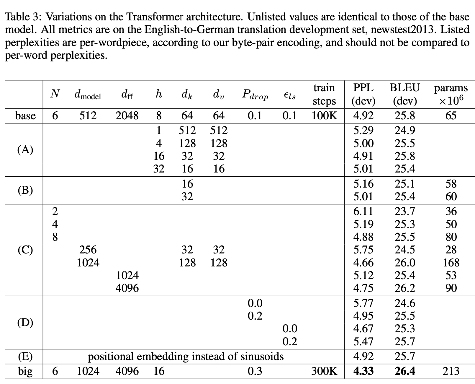Fig 10. Table. 3

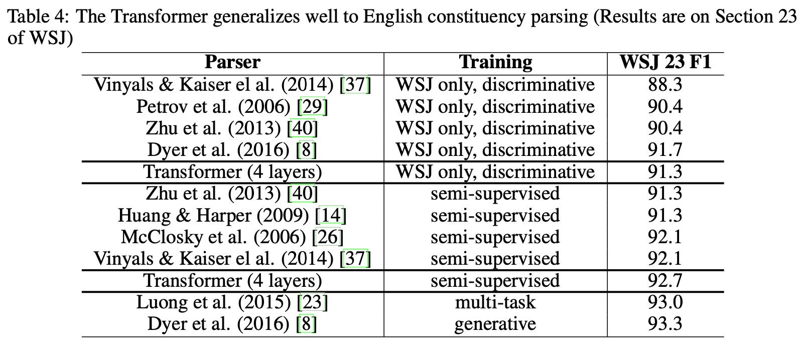Fig 11. Table. 4

Fig 9 - 11의 결과를 통해서 본 Transformer가 좋은 성능을 보이며 (English-to-German & English-to-French) English Consistuency Parsing에서도 별도의 튜닝 작업 없이도 좋은 성능을 보였다고 말합니다(Fig 11 참고).

" In contrast to RNN sequence-to-sequence models [37], the Transformer outperforms the Berkeley- Parser [29] even when training only on the WSJ training set of 40K sentences. "

Conclusion

Transformer의 등장으로 새로운 패러다임이 열렸다고 평가하는 부분이 많습니다. 그리고 현재까지도 다양한 응용이 이뤄지고 있습니다. 다음 포스트는 NLP 영역에서 사용되는 Transformer를 컴퓨터 비전에 적용한 ViT 논문에 대해 리뷰해보도록 하겠습니다.