신경망 넘파이로 만들어 보기

딥러닝 구조를 직접 넘파이 코딩으로 단순하게 만들어 보기

일단 keras에서 제공하는 mnist파일을 호출했습니다.

import tensorflow as tf
from tensorflow import keras
import numpy as np
import matplotlib.pyplot as plt

# MNIST 데이터를 로드. 다운로드하지 않았다면 다운로드까지 자동으로 진행됩니다. 
mnist = keras.datasets.mnist
(x_train, y_train), (x_test, y_test) = mnist.load_data()

x_train_norm, x_test_norm = x_train / 255.0, x_test / 255.0
x_train_reshaped = x_train_norm.reshape(-1, x_train_norm.shape[1]*x_train_norm.shape[2])
x_test_reshaped = x_test_norm.reshape(-1, x_test_norm.shape[1]*x_test_norm.shape[2])

신경망 구조에서 입력값이 들어가면 각각의 가중치를 곱하고 합하여 계산이 이뤄집니다. 행렬 연산의 특징을 이용하여 단순하게 시도할 것입니다.

• y = WX + B

# 테스트를 위해 x_train_reshaped의 앞 5개의 데이터를 가져온다.
X = x_train_reshaped[:5]
print(X.shape)

(5, 784)

weight_init_std = 0.1
input_size = 784
hidden_size=50

# 가중치는 랜덤한 값으로 하겠습니다.
W1 = weight_init_std * np.random.randn(input_size, hidden_size)  
# 편향 B는 일단 0으로 하겠습니다.
b1 = np.zeros(hidden_size)

a1 = np.dot(X, W1) + b1   # 은닉층 출력

print(W1.shape)
print(b1.shape)
print(a1.shape)

(784, 50)
(50,)
(5, 50)

위 코드를 통해 y = WX + b를 계산했습니다. a1의 결과를 확인해보겠습니다.

a1[0]

array([ 0.48653043, 1.21548756, 0.52309409, 0.93320544, -0.19513847,
1.28226922, 0.21049477, 0.24713435, 1.50274588, 0.31687977,

여기까지는 아직 퍼셉트론이라고 할 수 있고 신경망과 퍼셉트론의 차이인 활성화 함수를 곱하겠습니다. 여기서 할 활성화 함수는 시그모이드 입니다.

def sigmoid(x):
    return 1 / (1 + np.exp(-x))  


z1 = sigmoid(a1)
print(z1[0])

[0.61928875 0.77126847 0.62787098 0.71772515 0.4513696 0.7828358
0.55243025 0.56147104 0.81798366 0.57856364 0.78485329 0.48944915
0.34330287 0.3729736 0.40342849 0.38269088 0.46182855 0.72459828

시그모이드 함수를 통해 위에서 계산된 값들이 0~1값으로 변경되었습니다. 활성화 함수를 통해 비선형 적인 특성을 넣어 표현력이 더 강력하게 보완?한다고 생각해볼 수 있습니다.

지금까지 진행한 순방향 신경망 구조를 2층으로 쌓아 실행하는 코드를 만들어 보겠습니다.

1층 단위로 움직이는 함수를 먼저 만듭니다.

def affine_layer_forward(X, W, b):
    y = np.dot(X, W) + b
    cache = (X, W, b)
    return y, cache

아래 코드를 통해 W가중치 랜덤으로 설정해주고 B는 0입니다.

• 행렬의 특성상 곱이 이뤄질 수 있도록 shape를 맞춰야 한다는 점을 유의해야 합니다.

input_size = 784
hidden_size = 50
output_size = 10

W1 = weight_init_std * np.random.randn(input_size, hidden_size)
b1 = np.zeros(hidden_size)
W2 = weight_init_std * np.random.randn(hidden_size, output_size)
b2 = np.zeros(output_size)

a1, cache1 = affine_layer_forward(X, W1, b1)
z1 = sigmoid(a1)
a2, cache2 = affine_layer_forward(z1, W2, b2)    # z1이 다시 두번째 레이어의 입력이 됩니다. 

print(a2[0])

[ 0.00249933 0.01344503 -0.42532385 0.05259049 -0.70140225 0.58711998
-0.49198317 -0.30481471 0.30129486 0.56424935]

여기서는 softmax를 적용해보겠습니다. softmax는 0~1값으로 반환하고 반환한 값들을 모두 더하면 1이 되는 특성이 있습니다. 모든 손실을 포함시켜주는 역할을 합니다.

def softmax(x):
    if x.ndim == 2:
        x = x.T
        x = x - np.max(x, axis=0)
        y = np.exp(x) / np.sum(np.exp(x), axis=0)
        return y.T 

    x = x - np.max(x) # 오버플로 대책
    return np.exp(x) / np.sum(np.exp(x))

y_hat = softmax(a2)
y_hat[0]

array([0.09568883, 0.09674197, 0.0623821 , 0.10060408, 0.04733264,
0.17169545, 0.05835932, 0.07037145, 0.12901093, 0.16781323])

softmax를 통해 값을 얻었다면 가장 큰값을 얻는 값이 정답이게 됩니다. 하지만 신경망에서는 여기서 그치지 않고 이 손실값을 통해 앞에서 계산해왔던 가중치들을 수정해줍니다. 그러기 위해서 loss function을 사용합니다. 여기서는 cross entropy를 사용하겠습니다.

cross entropy란 두 확률분포 사이에서 유사도가 높을 수록 그 차이는 작아 집니다. 또한 각 정답과의 차이를 entropy함수에 소프트맥스값을 넣어 불순도를 측정합니다. 이 정답을 답으로 했을때의 불안한 정도를 값으로 표현한다고 생각하면 될 것 같습니다.

• [http://www.gisdeveloper.co.kr/?p=7631 참고
  cross enropy를 사용하기 위해서는 0과 1로 label을 표현하도록 원핫 인코딩을 해야합나다.

def _change_one_hot_label(X, num_category):
    T = np.zeros((X.size, num_category))
    for idx, row in enumerate(T):
        row[X[idx]] = 1
        
    return T

Y_digit = y_train[:5]
t = _change_one_hot_label(Y_digit, 10)
t

array([[0., 0., 0., 0., 0., 1., 0., 0., 0., 0.],
[1., 0., 0., 0., 0., 0., 0., 0., 0., 0.],
[0., 0., 0., 0., 1., 0., 0., 0., 0., 0.],
[0., 1., 0., 0., 0., 0., 0., 0., 0., 0.],
[0., 0., 0., 0., 0., 0., 0., 0., 0., 1.]])

cross entropy식에 맞게 정의를 해주고 loss값을 찾습니다.

def cross_entropy_error(y, t):
    if y.ndim == 1:
        t = t.reshape(1, t.size)
        y = y.reshape(1, y.size)
        
    # 훈련 데이터가 원-핫 벡터라면 정답 레이블의 인덱스로 반환
    if t.size == y.size:
        t = t.argmax(axis=1)
             
    batch_size = y.shape[0]
    return -np.sum(np.log(y[np.arange(batch_size), t])) / batch_size

Loss = cross_entropy_error(y_hat, t)
Loss

2.2142990931042563

batch_num = y_hat.shape[0]
dy = (y_hat - t) / batch_num
dy

rray([[ 0.01913777, 0.01934839, 0.01247642, 0.02012082, 0.00946653,
-0.16566091, 0.01167186, 0.01407429, 0.02580219, 0.03356265],

파라미터 W의 변화에 따른 오차(Loss) L의 변화량을 구해보겠습니다.

batch_num = y_hat.shape[0]
dy = (y_hat - t) / batch_num
dy

array([[ 0.01913777, 0.01934839, 0.01247642, 0.02012082, 0.00946653,
-0.16566091, 0.01167186, 0.01407429, 0.02580219, 0.03356265],

[https://deepnotes.io/softmax-crossentropy]

기울기를 시그모이드를 통해 나온 값에 dy 변화량을 곱하겠습니다.

dW2 = np.dot(z1.T, dy)    
dW2

모든 파라미터 W1, b1, W2, b2에 대한 기울기

dW2 = np.dot(z1.T, dy)
db2 = np.sum(dy, axis=0)

중간중간 마다 시그모이드를 사용하기 때문에 활성화 함수에 대한 gradient도 고려합니다.

def sigmoid_grad(x):
    return (1.0 - sigmoid(x)) * sigmoid(x)

dz1 = np.dot(dy, W2.T)
da1 = sigmoid_grad(a1) * dz1
dW1 = np.dot(X.T, da1)
db1 = np.sum(dz1, axis=0)

파라미터 업데이트하는 함수를 생각해서 learning_rate도 고려합니다.

learning_rate = 0.1

def update_params(W1, b1, W2, b2, dW1, db1, dW2, db2, learning_rate):
    W1 = W1 - learning_rate*dW1
    b1 = b1 - learning_rate*db1
    W2 = W2 - learning_rate*dW2
    b2 = b2 - learning_rate*db2
    return W1, b1, W2, b2

backward 함수를 만들어서 한 사이클을 만들어 보겟습니다

def affine_layer_backward(dy, cache):
    X, W, b = cache
    dX = np.dot(dy, W.T)
    dW = np.dot(X.T, dy)
    db = np.sum(dy, axis=0)
    return dX, dW, db

# 파라미터 초기화
W1 = weight_init_std * np.random.randn(input_size, hidden_size)
b1 = np.zeros(hidden_size)
W2 = weight_init_std * np.random.randn(hidden_size, output_size)
b2 = np.zeros(output_size)

# Forward Propagation
a1, cache1 = affine_layer_forward(X, W1, b1)
z1 = sigmoid(a1)
a2, cache2 = affine_layer_forward(z1, W2, b2)

# 추론과 오차(Loss) 계산
y_hat = softmax(a2)
t = _change_one_hot_label(Y_digit, 10)   # 정답 One-hot 인코딩
Loss = cross_entropy_error(y_hat, t)

print(y_hat)
print(t)
print('Loss: ', Loss)
        
dy = (y_hat - t) / X.shape[0]
dz1, dW2, db2 = affine_layer_backward(dy, cache2)
da1 = sigmoid_grad(a1) * dz1
dX, dW1, db1 = affine_layer_backward(da1, cache1)

# 경사하강법을 통한 파라미터 업데이트    
learning_rate = 0.1
W1, b1, W2, b2 = update_params(W1, b1, W2, b2, dW1, db1, dW2, db2, learning_rate)

[[0.07850856 0.05053692 0.22863595 0.08858019 0.10341642 0.07413686
0.15236807 0.08707045 0.06696473 0.06978184][0.07063963 0.05589779 0.22244935 0.09845158 0.09501542 0.07559829 0.15462916 0.08653334 0.07542828 0.06535716]
[0.06562364 0.07036418 0.1837287 0.09718998 0.12400164 0.07974449
0.13354298 0.09022088 0.09394088 0.06164263][0.06374149 0.06032105 0.19419075 0.1038898 0.10028428 0.06944635 0.18646018 0.08004788 0.08655625 0.05506198]
[0.0527867 0.055662 0.20487245 0.1102281 0.12172459 0.06421484
0.18759931 0.07394098 0.0826122 0.04635883]]
[[0. 0. 0. 0. 0. 1. 0. 0. 0. 0.][1. 0. 0. 0. 0. 0. 0. 0. 0. 0.]
[0. 0. 0. 0. 1. 0. 0. 0. 0. 0.][0. 1. 0. 0. 0. 0. 0. 0. 0. 0.]
[0. 0. 0. 0. 0. 0. 0. 0. 0. 1.]]
Loss: 2.6437769325086995

softmax와 정답 라벨의 one hot 인코딩의 분포가 유사해지기를 기대합니다.

위의 과정을 한 코딩에 해보겠습니다.

W1 = weight_init_std * np.random.randn(input_size, hidden_size)
b1 = np.zeros(hidden_size)
W2 = weight_init_std * np.random.randn(hidden_size, output_size)
b2 = np.zeros(output_size)

def train_step(X, Y, W1, b1, W2, b2, learning_rate=0.1, verbose=False):
    a1, cache1 = affine_layer_forward(X, W1, b1)
    z1 = sigmoid(a1)
    a2, cache2 = affine_layer_forward(z1, W2, b2)
    y_hat = softmax(a2)
    t = _change_one_hot_label(Y, 10)
    Loss = cross_entropy_error(y_hat, t)

    if verbose:
        print('---------')
        print(y_hat)
        print(t)
        print('Loss: ', Loss)
        
    dy = (y_hat - t) / X.shape[0]
    dz1, dW2, db2 = affine_layer_backward(dy, cache2)
    da1 = sigmoid_grad(a1) * dz1
    dX, dW1, db1 = affine_layer_backward(da1, cache1)
    
    W1, b1, W2, b2 = update_params(W1, b1, W2, b2, dW1, db1, dW2, db2, learning_rate)
    
    return W1, b1, W2, b2, Loss

X = x_train_reshaped[:5]
Y = y_train[:5]

# train_step을 다섯 번 반복 돌립니다.
for i in range(5):
    W1, b1, W2, b2, _ = train_step(X, Y, W1, b1, W2, b2, learning_rate=0.1, verbose=True)

5번 학습한 파라미터를 바탕으로 정확도를 측정해보겠습니다.

def predict(W1, b1, W2, b2, X):
    a1 = np.dot(X, W1) + b1
    z1 = sigmoid(a1)
    a2 = np.dot(z1, W2) + b2
    y = softmax(a2)

    return y

# X = x_train[:100] 에 대해 모델 추론을 시도합니다. 
X = x_train_reshaped[:100]
Y = y_test[:100]
result = predict(W1, b1, W2, b2, X)
result[0]

array([0.15564588, 0.1326148 , 0.03664334, 0.05631935, 0.1105738 ,
0.19383691, 0.04018136, 0.0572725 , 0.03751335, 0.17939871])

def accuracy(W1, b1, W2, b2, x, y):
    y_hat = predict(W1, b1, W2, b2, x)
    y_hat = np.argmax(y_hat, axis=1)

    accuracy = np.sum(y_hat == y) / float(x.shape[0])
    return accuracy
acc = accuracy(W1, b1, W2, b2, X, Y)

t = _change_one_hot_label(Y, 10)
print(result[0])
print(t[0])
print(acc)

[0.15564588 0.1326148 0.03664334 0.05631935 0.1105738 0.19383691
0.04018136 0.0572725 0.03751335 0.17939871][0. 0. 0. 0. 0. 0. 0. 1. 0. 0.]
0.06

아직 정확도는 10%도 안되는 정도로 나왔습니다.. 여러번 반복이 필요하겠죠,,?

def init_params(input_size, hidden_size, output_size, weight_init_std=0.01):

    W1 = weight_init_std * np.random.randn(input_size, hidden_size)
    b1 = np.zeros(hidden_size)
    W2 = weight_init_std * np.random.randn(hidden_size, output_size)
    b2 = np.zeros(output_size)

    print(W1.shape)
    print(b1.shape)
    print(W2.shape)
    print(b2.shape)
    
    return W1, b1, W2, b2

10000번을 반복해보겠습니다 5번보다는 확실히 많이 반복하게됩니다.

# 하이퍼파라미터
iters_num = 10000  # 반복 횟수를 적절히 설정한다.
train_size = x_train.shape[0]
batch_size = 100   # 미니배치 크기
learning_rate = 0.1

train_loss_list = []
train_acc_list = []
test_acc_list = []

# 1에폭당 반복 수
iter_per_epoch = max(train_size / batch_size, 1)

W1, b1, W2, b2 = init_params(784, 50, 10)

for i in range(iters_num):
    # 미니배치 획득
    batch_mask = np.random.choice(train_size, batch_size)
    x_batch = x_train_reshaped[batch_mask]
    y_batch = y_train[batch_mask]
    
    W1, b1, W2, b2, Loss = train_step(x_batch, y_batch, W1, b1, W2, b2, learning_rate=0.1, verbose=False)

    # 학습 경과 기록
    train_loss_list.append(Loss)
    
    # 1에폭당 정확도 계산
    if i % iter_per_epoch == 0:
        print('Loss: ', Loss)
        train_acc = accuracy(W1, b1, W2, b2, x_train_reshaped, y_train)
        test_acc = accuracy(W1, b1, W2, b2, x_test_reshaped, y_test)
        train_acc_list.append(train_acc)
        test_acc_list.append(test_acc)
        print("train acc, test acc | " + str(train_acc) + ", " + str(test_acc))

마지막으로 훈련과정을 그래프로 보면 더 편하게 확인할 수 있습니다. Loss와 accuracy의 변화를 시각화 하겠습니다.

# Loss 그래프 그리기
x = np.arange(len(train_loss_list))
plt.plot(x, train_loss_list, label='train acc')
plt.xlabel("epochs")
plt.ylabel("Loss")
plt.ylim(0, 3.0)
plt.legend(loc='best')
plt.show()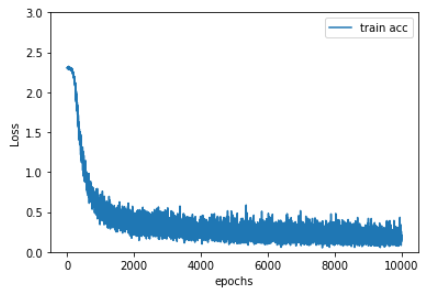

간단한 신경망 구조를 행렬계산을 통해 확인했습니다. Mnist는 신경망으로 분석을 하기 정말 좋은 모양을 하기 때문에 간단한 신경망 구조로도 좋은 정확도를 가질 수 있었습니다.

모두연구소 AIFFEL 우지철님이 만들어주신 교육 참고입니다! (메일이 없어서,,, 따로 연락망을 공유를 못하네요,,ㅜ