Decision Trees

‍이세현·2024년 6월 11일

Introduction to Machine Learning

Task: Classification
빠르고 정확하다

Machine Learning

Machine Learning: Data 기반 Function Approximation

Problem Setting

Learning Type: Supervised Learning
Instances: $x$ , Labels: $y$
Unknown target function: $f:x \rightarrow y$
Function Hypothesis: $H=\{h|h:x \rightarrow y\}$
Output: $f$ 에 가장 근사한 가설 $h \in H$

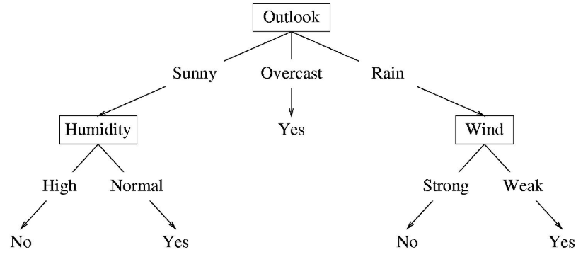
Sample Dataset

Outlook, Temperature, Humidity, Wind에 따른 Class 여부

Decision Tree

Neural Network와 다른 점

Parameter 연산 없이 Feature만으로 출력을 결정한다.
Neural Network는 Feature에 내제된 것을 계산하므로 표현력이 더 좋다.

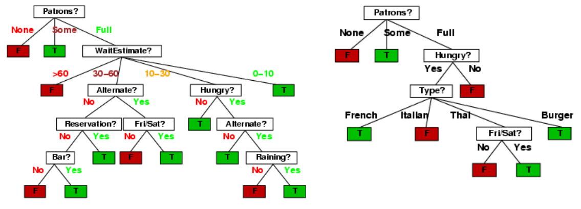
Decision Tree

if-else 형태 - 지나치게 많아지면 Tree 사용이 어렵다.
- 이미지의 경우 256*256 pixel에 대해 가지가 생성된다.
Internal Node: test one attribute $X_i$
Branch from a node: $X_i$ 선택
Leaf node: predict $Y$
위의 예에서 Temperature node는 없다. Attribute가 Node로 사용되지 않을 수 있다.
Prediction Sample
- Data: <outlook=sunny, temperature=hot, humidity=high, wind=weak>
- Prediction: No

연속적인 속성에 대한 Decision Tree

Internal node는 threshold에 대해 feature의 값을 test할 수 있다.

Decision Tree Learning

Problem Setting
- Instances: $x$ , Labels: $y$
  - 각 instance $x$ 는 feature vectore $X$ 에 해당한다.
  - $x$ 는 low, high 등 instance
- Unknown target function: $f:x \rightarrow y$
  - $Y$ 는 이산 변수이다.
- Function Hypothesis: $H=\{h|h:x \rightarrow y\}$
  - 각 가설 $h$ 는 decision tree
  - tree는 $x$ 를 y로 할당되는 leaf로 분류한다.
- Output: $f$ 에 가장 근사한 가설 $h \in H$

Decision Tree Machine Learning

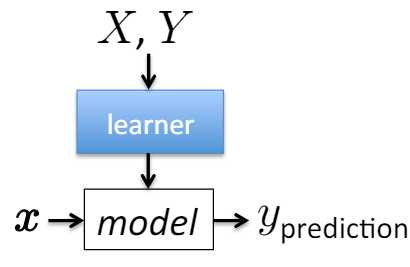
다른 머신러닝 알고리즘과 동일하게 학습한다.

Given: labeled training data $X, Y$
Train: $\text{model} \leftarrow \text{classifier.train}(X,Y)$
Apply to new data
- Given: unlabled instance
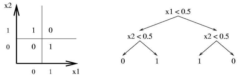
- $y_\text{prediction} \leftarrow \text{model.predict}(X)$

Decision Boundary

Decision Tree는 feature space를 축에 평행하게 분할한다.
각 직사각형 영역은 하나의 label이거나 label에 대한 확률 분포이다.

Expressiveness

Decision tree는 모든 binary 문제를 풀 수 있다.
최악의 경우, tree는 exponentially 많은 node를 필요로 한다.
Decision tree는 변수만큼의 hypothesis space를 가진다.
- Node의 개수가 늘어날수록 hypothesis 공간이 커진다.
- Depth 1(decision stump): feature의 모든 boolean function을 나타낼 수 있다.
  - 하나의 feature로 분류하는 root
- Depth 2: 두개의 feature를 가진 boolean function
  
  문제점: 심각한 Overffiting. Test Data를 보장할 수 없다.

Preference bias: Ockham's Razor

Tree 역시 가장 간단할수록 좋다.

모든 training data를 정확하게 분류하는 가장 작은 decision tree가 가장 최선이다.

Basic Algorithm for Top-Down Induction of Decision Trees

node = Decision tree의 root
Main Loop
1. A $\leftarrow$ 최선의 decision attribute
2. Node에 대한 decision attribute로 A 할당
3. A 각각에 대해 새로운 자식 node를 만든다.
4. Training examples를 leaf node로 배정한다.
5. Training examples가 완벽히 분류되었다면 그만한다.
  그렇지 않으면 새로운 leaf node에 대해 반복한다.

최선의 Attribute를 선택하는 방법

어느 attribute가 examples를 가장 잘 나누는지 알아야 한다.
Possibilities
- Random: Attribute를 무작위로 선택한다.
- Least-Values: 가장 적은 가지를 만드는 Attribute를 선택한다.
- Most-Values: 가장 많은 경우를 만들어내는 Attribute를 선택한다.
- Max-Gain: Information gain이 가장 큰 Attribute를 선택한다.
  ID# algorithm은 Max-Gain method를 사용한다.
Idea: 가장 좋은 Attribute는 examples를 "all positive" 또는 "all negative"로 분류한다.

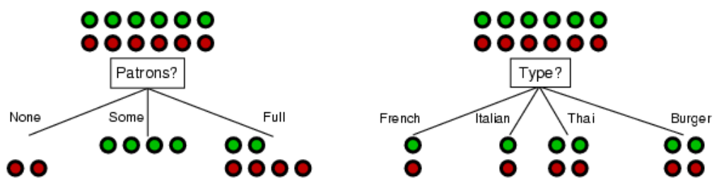
Patron으로 구분한 경우 examples가 완벽하게 갈린다.
- Compare Example
- Examples가 완벽하게 갈릴수록 정보적 이득이 크다.

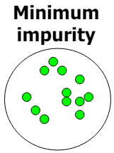
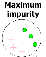
Impurity/Entropy (informal)

Example 그룹에서 Impurity(불순) 정도를 계산한다.
Entropy: impurity를 측정하는 일반적인 방법
$H(X)=-\sum{P(X=i)\log_2P(X=i)}$
- Probability와 probability의 bit 개수
- $H(X)$ 는 $X$ 값을 인코딩하는 데 필요한 예상 Bit 개수이다.
  - 가장 효율적인 코드는 $X=i$ 라는 메시지를 인코딩하기 위해 $-\log_2P(X=i)$ bit를 사용한다.
  - 가장 효율적인 코드: 최소한의 비트로 메시지를 인코딩하는 것
  - $-\log_2{P(X=i)}$ bit: 정보량을 측정하는 단위. $P(X=i)$ 가 작을수록 정보량이 많아지고 더 많은 비트가 필요하다.
  - 특정 사건이 발생할 확률에 따라 bit를 할당하면 평균적으로 가장 적은 비트 수로 정보를 인코딩할 수 있다.
  - Random 사건 $X$ 에 필요한 bit 수 $\sum_{i=1}^{n}P(X=i)(-\log_2P(X=i))$
Huffman code

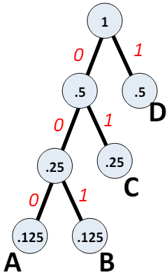
빈도수가 낮은 A와 B는 더 많은 bit를 사용하고
빈도수가 높은 C와 D는 더 적은 bit를 사용하여
bit 낭비를 줄인다.

M code length probability 정보량
A 000 3 0.125 0.375
B 001 3 0.125 0.375
C 01 2 0.250 0.500
D 1 1 0.500 0.500
Total Average Bits/message 1.750

M	code	length	probability	정보량
A	000	3	0.125	0.375
B	001	3	0.125	0.375
C	01	2	0.250	0.500
D	1	1	0.500	0.500
Total			Average Bits/message	1.750

2-Class Cases


모든 샘플이 하나의 클래스에 속하는 경우	샘플이 50% 비율로 섞여있는 경우
$P(X=i)=1$	$P(X=i)=0.5, P(X=j)=0.5$
정보량: $\log_2P(X=i)=0$	정보량: $-1, -1$
$H(X)=0$	$H(X)=1$

Sample Entropy

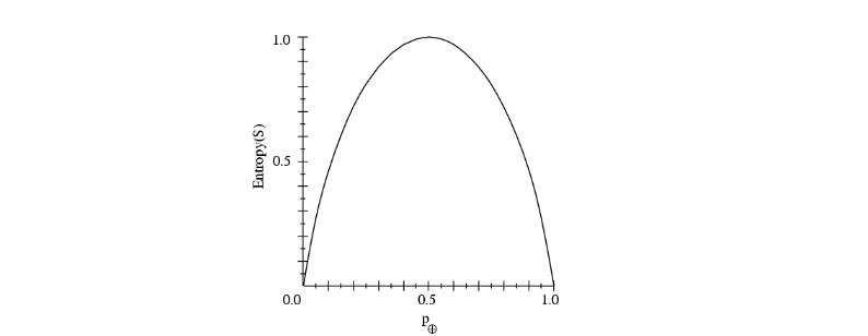
$S$ : Training examples 샘플
$S$ 의 impurity를 나타내는 Entropy $H(S)=-p_\oplus\log_2{p_\oplus}-p_\ominus\log_2{p_\ominus}$
Entropy가 가장 클 때
- $p_\oplus$ 와 $p_\ominus$ 는 각각 50%로 섞여있다.
- 불확실성이 크다.
- 정보량이 낮다. 얻을 수 있는 정보가 없다.
- 데이터가 pure 할수록 entropy가 낮다.

Information Gain

Training feature vector에서 어떤 속성이 분류하기에 가장 효율적인지(impurity가 작은지) 결정해야 한다.
Information Gain은 주어진 feature vector의 속성이 얼마나 중요한지 나타낸다.
- Decision tree의 node에서 attribute의 속성을 결정하는 데 사용된다.

From Entropy to Infromation Gain

조건부 entropy (given $Y=v$ )
$H(X|Y=v)=-\sum_{i=1}^{n}P(X=i|Y=v)\log_2({X=i|Y=v})$
- $Y=v$ : Attribute가 $v$ 로 고정된 것을 의미한다.
- $v$ 가 여러개이면 각 $v$ 에 대해 계산 후 마지막에 합한다.
  - $H(X|Y)=\sum_{v\in\text{values}(Y)}P(Y=v)H(X|Y=v)$
- Mututal(상호) information = Information Gain
  $I(X,Y)=H(X)-H(X|Y)=H(Y)-H(Y|X)$
  - $H(X)$ 는 클수록 불확실성이 높다.
  - $H(X)$ : 확률 변수 $X$ 의 엔트로피, 즉 $X$ 의 불확실성을 나타낸다.
  - $H(X∣Y)$ : $Y$ 가 주어졌을 때의 $X$ 의 조건부 엔트로피, 즉 $Y$ 를 알고 있을 때 남아 있는 $X$ 의 불확실성을 나타낸다.
  - $Y$ 가 주어졌을 때 $X$ 의 불확실성이 얼마나 낮아지는지 설명한다.
  - 만약 두 변수가 독립이라면 $Y$ 를 알아도 $X$ 의 불확실성은 낮아지지 않으므로 $H(X|Y)=H(X)$ 이 되어 $I(X,Y)=0$ 이 된다.
  - $Y$ 가 $X$ 를 완전히 결정한다면 $I(X,Y)=1$ 이 된다.
    $I(X,Y)$ 는 클수록 좋다.
  - $I(X,Y)$ 는 두 변수가 서로 얼마나 많은 정보를 공유하는지 나타낸다.
Information Gain 계산
Information Gain = Entropy(parent) - Average Entropy(Children)
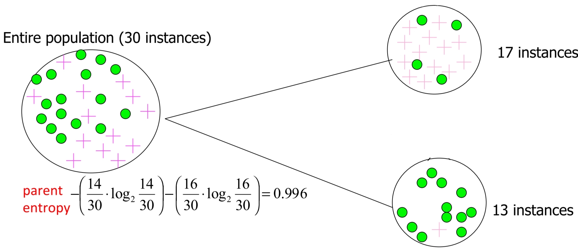
- Child Entropy
  - 17 Instances: $-\frac{4}{17}\cdot\log_2\frac{4}{17}-\frac{13}{17}\cdot\log_2\frac{13}{17} = 0.787$
  - 13 Instances: $-\frac{12}{13}\cdot\log_2\frac{12}{13}-\frac{1}{13}\cdot\log_2\frac{1}{13} = 0.391$
- Weighted Average Entropy of Children
  $\frac{17}{30}\cdot0.787+\frac{13}{30}\cdot0.391=0.615$
- Information Gain
  $0.996 - 0.615 = 0.38$
- 모든 Attribute에 대해 계산한 후 최종 선택한다.
Disadvantage of Information Gain
- 데이터를 작은 pure 집합으로 분할하는 많은 값을 가진 속성을 선택하게 된다.
- 다중값 속성에 대한 편향으로 이어질 수 있다.
- 이를 개선하기 위해 Quinlan's gain ratio를 사용하여 정규화를 도입한다.