Neural Networks: Representation

Non-linear hypothesis

Non-linear Classification

• $x$에 대해 비선형적 decision boundary를 구해야 할 때 매우 많은 features 조합이 필요하다.
  • logistic regression은 feature의 수가 많아질수록 식을 위해 필요한 항이 매우 많아지고 overfitting이 발생할 수도 있다.
• 입력이 $50 \times 50 \times 1$ 이미지인 경우 pixel 수는 2500, quadratic features만 $_{2500}\mathrm{ C }_{2} \approx 3000000$로 경우가 매우 많아진다.
  • 위의 경우 Logistic regression 같은 non-linear classification은 좋은 해결 방법이 아니다.
  • 이를 해결하기 위해 더욱 효율적인 neural network가 등장하였다.

Neurons and the brain

Neural Networks

• Origins: 뇌를 모방한 algorithms
• 80~90년대에 광범위하게 사용되었다.
  • 90년대 후반부터 덜 사용되지 시작하였다.
• 최근 재기: 많은 영역에서 사용하는 최신 기술

Model representation

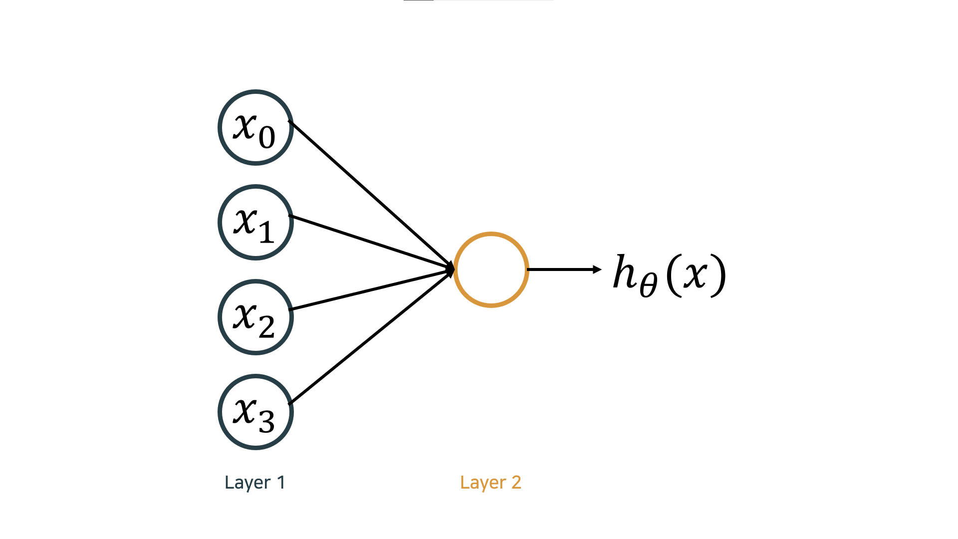
Neuron model: Logistic unit

• $x$: 입력 신호 unit, $\theta$: parameters/weights
  $x=\begin{bmatrix} x_0 \\ x_1 \\ x_2 \\ x_3 \end{bmatrix}, \theta=\begin{bmatrix} \theta_0 \\ \theta_1 \\ \theta_2 \\ \theta_3 \end{bmatrix}$
• layer: parameter 기준이 아닌 data 기준으로 count
• layer 1: unit 세 개로 이루어진 layer

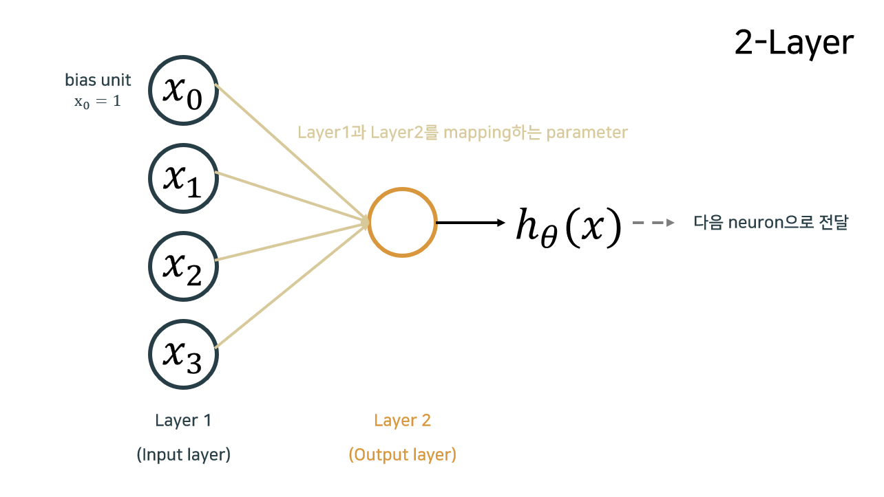
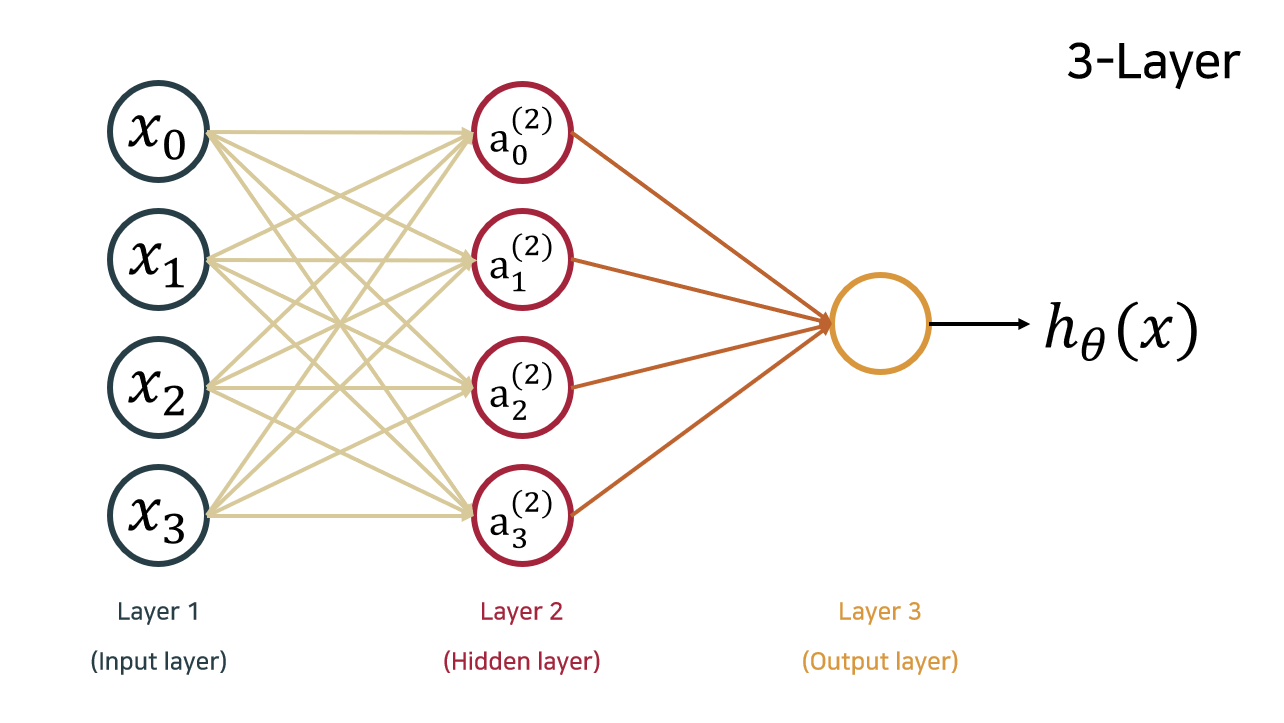
Neural Network

hiddne layer를 중첩하는 구조이다.

$x$에서 $a_0$은 연결하지 않는다.

• Hidden layer: 눈에 보이는 input, output layer와 달리 보이지 않는 중간 layer
• $a_i^{(j)}$: layer $j$의 $i$ unit의 activation
• $\theta^{(j)}$: layer $j$와 layer $j+1$을 연결하는 mapping matrix
  $a_1^{(2)}=g(\theta_{10}^{(1)}x_0 + \theta_{11}^{(1)}x_1 + \theta_{12}^{(1)}x_2 + \theta_{13}^{(1)}x_3) \\ a_2^{(2)}=g(\theta_{20}^{(1)}x_0 + \theta_{21}^{(1)}x_1 + \theta_{22}^{(1)}x_2 + \theta_{23}^{(1)}x_3) \\ a_3^{(2)}=g(\theta_{30}^{(1)}x_0 + \theta_{31}^{(1)}x_1 + \theta_{32}^{(1)}x_2 + \theta_{33}^{(1)}x_3)$
  • $g$: non linear activation function
• layer $j$에 $s_j$ units이 있고, layer $j+1$에 $s_{j+1}$ units이 있다면
  • $\theta^{(j)}$의 크기는 $s_{j+1} \times (s_j+1)$이다.
  • $+1$: 이전 unit의 bias

Forward propagation: Vectorized implementation

• Forward propagation: 연산 이후 다음 layer로 전달하는 과정
  • 학습 시에는 backward propagation
• linear parameter $\theta$를 아무리 중첩하여도 linear layer 하나 곱한 것과 동일한 효과
  • $z^{(2)}=\theta^{(1)}a^{(1)}$
  • $a^{(2)}=g(z^{(2)})$
  • $h_\theta(x)=a^{(3)}=g(z^{(3)})$

Neural Network learning its own features

data $x$를 통해 $\theta$를 구해야 한다.

• 올바른 $\theta$를 구하기 위해서는 좋은 data가 필요하다.

Examples and intuitions

Non-linear classification example: XOR/XNOR

$x1$, $x2$가 0 or 1(binary)

• $y=x_1 \text{ XOR }x_2$

  • 일차함수로 구분할 수 없다.

    $x1$	$x2$	y
    0	0	1
    0	1	0
    1	1	0
    1	1	1

• $y=x_1 \text{ XNOR }x_2 \\ \text{NOT } (x_1 \text{ XOR }x_2)$
  

Simple example: AND

• $y=x_1 \text{ AND } x_2$

  • $\theta=\begin{bmatrix} -30 & 20 & 20 \end{bmatrix}$

  • $h_\theta(x)=g(-30+20x_1+20x_2)$

    $x_1$	$x_2$	$h_\theta(x)$
    0	0	$g(-30) \approx 0$
    0	1	$g(-10) \approx 0$
    1	0	$g(-10) \approx 0$
    1	1	$g(10) \approx 1$

Example: OR function

• $y=x_1 \text{ OR } x_2$

  • $\theta=\begin{bmatrix} -10 & 20 & 20 \end{bmatrix}$

  • $h_\theta(x)=g(-10+20x_1+20x_2)$

    $x_1$	$x_2$	$h_\theta(x)$
    0	0	$g(-10) \approx 0$
    0	1	$g(10) \approx 1$
    1	0	$g(10) \approx 1$
    1	1	$g(30) \approx 1$

XOR function - Neural Network

$x_1$	$x_2$	$\text{AND}$	$\text{NOR}$	$a_0 \text{ OR } a_1$
0	0	0	1	1
0	1	0	0	0
1	0	0	0	0
1	1	1	0	1

Multi-class classification

• logistic regression의 경우 binary classification N개 중 가장 확률이 큰 값을 prediction으로 출력하였다.
• Neural network의 경우 단 하나의 모델로 표현 가능하다.

  one-hot encoding

  • when answer 0
    $h_\theta(x) \approx \begin{bmatrix} 1 \\ 0 \\ 0 \\ 0 \end{bmatrix}$
  • when answer 1
    $h_\theta(x) \approx \begin{bmatrix} 0 \\ 1 \\ 0 \\ 0 \end{bmatrix}$