regression

='regression toward the mean'
결과적으로 데이터는 평균으로 회귀한다

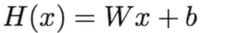
선형회귀

y_data =[1,2,3,4,5]

W=tf.Variable(2,9)
b=tf.Variable(0.5)

hypothesis=W * x_data + b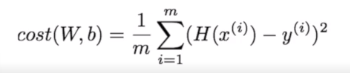

cost = tf.reduce_mean(tf.square(hypothesis - y_data))
#square= 제곱
#reduce_mean =차원축소 평균

Gradient descent (경사하강 알고리즘)

: W,b를 찾아 비용의 최소를 구하는 알고리즘

learning_rate=0.01

# W,b값을 여러 차례 구하기
for i in rage (100+1):

#변수(W,b)정보를 tape에 기록
with tf.GradientTape() as tape :
	hypothesis = W * x_data +b
    cost = tf.reduce_mean(tf.square(hypothsis - y_data))

#gradient 경사값(미분값) 구하기
W_grad, b_grad = tape.gradient(cost, [W,b])

#assign_sub -> A= A-B      A-=B
W.assign_sub(learning_rate * W_grad)
b.assign_sub(learning_rate * b_grad)

if i %10 ==0:

간략화된 가설함수

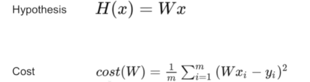
함수 식

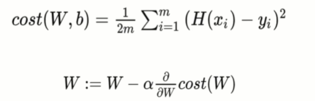
a값은 얼마만큼 변경할지 결정하는 파라미터

코드

#간략화된 가설함수 코드
import numpy as np

X= np.array([1,2,3])
Y= np.array([1,2,3])

def cost_func(W,X,Y):
	c=0
    for i in range(len(X)):
    	c+=(W*X[i] - Y[i])**2
     return c / len(X)

# -3부터 5사이를 15개 구간으로 나눠서 feed_W에 존재
#feed_W값에 따라 curr_cost값 바뀜

for feed_W in np.linspace(-3,5,num=15):
	curr_cost = cost_func(feed_W,X,Y)
    print("{:6.3f}|{:10.5f}".format(feed_W,curr_cost))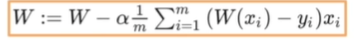

# 랜덤 seed 초기화(코드 다시 수행했을 때도 동일하게 재현하기 위해)
tf.set_random_seed(0)

x_data =[1.,2.,3.,4.]
y_data =[1.,3.,5.,7.]

#정규분포 1개 (W값이 무엇이든 0으로 수렴하게 됨)
W= tf.Variable(tf.random_nomal([1],-100.,100.))

for step in range(300):
	hypothesis = W * X
    cost = tf.reduce_mean(tf.square(hypothesis - Y )
    
    alpha = 0.01
    gradient = tf.reduce_mean(tf.multiply(tf.multiply(W,X)-Y, X))
    descent = W - tf.multiply(alpha,gradient)
    W.assing(descent)
    
# 10번에 한 번씩 출력
    if step % 10 ==0:
    	print('{:5} | {:10.4f} | {:10.6f}'.format(step,cost.numpy(),W.numpy()[0]))

다중 선형회귀

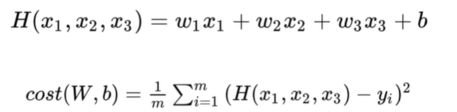
변수 값 만큼 가중치 갯수도 늘어남

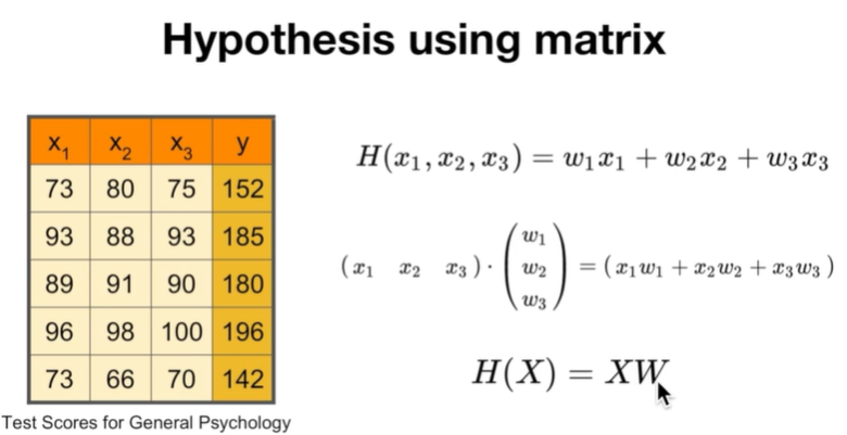
매트릭스를 이용하여 간편하게 기술

코드

#data 행렬식 준비

data = np.array([
	#X1   X2   X3   y
    [73.,80.,75.,152.],
    [93.,88.,93.,185.],
    [89.,91.,90.,180.],
    [96.,98.,100.,196.],
    [73.,66.,70.,142.],], dtype=np.float32)
    
#데이터 슬라이싱 ()
X= data[:,:-1]
y= data[:,[-1]]

# W는 3x1행렬 (3= x의 컬럼 갯수)
W= tf.Variable(tf.random_nomal([3,1]))
b= tf.Variable(tf.random_namal([1]))

#작은 상수값 지정
learning_rate = 0.00001

def predict(X):
	return tf.matmul(X,W) +b
    
n_epochs =2000
for i in range(n_epochs+1):
	with tf.GradientTape() as tape:
    	cost = tf.reduce_mean((tf.square(predicta(X)-y)))
        
    W_grad, b_grad = tape.gradient(cost,[W,b])
    
    #w, b값 계속 순회
    W.assign_sub(learning_rate * W_grad)
    b.assign_sub(learning_rate * b_grad)
    
    if i %100 ==0:
    	print("{:5} | {:10.4f}".format(i, cost.numpy()))
        

소프트맥스 (Softmax)

XW=Y (로지스틱 분류)

socres --> 소프트맥스 함수 --> 확률값

코드

tf.matmaul(X,W)+b
hypothesis= tf.nn.softmax(tf.matmul(X,W)+b)

비용함수 : 크로스 엔트로피(Cross-entropy)

• 예측값과 실제값의 차이를 확인하기 위함.

Y= log(Y_hat)
예측 함수 : Si #확률
실제 값: Li # 0 or 1

크로스 엔트로피 함수 : -시그마Li*log(Si)

함수

#corss entropy 값
cost= tf.reduce_mean(-tf.reduce_sum(Y*tf.log(hypothesis), axis=1))
optimizer= tf.train.GradientDescentOptimizer(learning_rate=0.1).minimize(cost)