
해당 글은 제로베이스데이터스쿨 학습자료를 참고하여 작성되었습니다
신용 카드 부정 사용자 검출
개요
- 신용카드 사기 검출 분류 실습용 데이터
- 데이터에 class라는 이름의 컬럼이 사기 유뮤를 의미
- class 컬럼의 불균형이 극심해서 전체 데이터의 약 0.172%가 1(사기 Fraud)을 가짐
목표
- 신용카드 부정 사용자 검출하기
절차
- 1) 데이터 이해
- 2) 단순 무식한 첫 도전 - 1st Trial
- 3) 데이터를 정리해서 다시 도전하자- 2nd Trial
- 4) 다시 데이터의 Outlier를 정리해보자- 3rd Trial
- 5) SMOTE Oversampling - 4th Trial
- 6) 학습내용 요약
1) 데이터 이해
데이터 특성
- 금융데이터이고 기업의 비밀보호를 위해 대다수의 특성이름은 삭제
- Amount : 거래금액
- Class : Fraud 여부(1이면 Fraud)
import pandas as pd

data_path = './data/creditcard.csv'
raw_data = pd.read_csv(data_path)
raw_data.head()
raw_data.columns
-----------------------------------------------------------------------------
   Time        V1        V2        V3        V4        V5        V6        V7  \
0   0.0 -1.359807 -0.072781  2.536347  1.378155 -0.338321  0.462388  0.239599
1   0.0  1.191857  0.266151  0.166480  0.448154  0.060018 -0.082361 -0.078803
2   1.0 -1.358354 -1.340163  1.773209  0.379780 -0.503198  1.800499  0.791461
3   1.0 -0.966272 -0.185226  1.792993 -0.863291 -0.010309  1.247203  0.237609
4   2.0 -1.158233  0.877737  1.548718  0.403034 -0.407193  0.095921  0.592941

         V8        V9  ...       V21       V22       V23       V24       V25  \
0  0.098698  0.363787  ... -0.018307  0.277838 -0.110474  0.066928  0.128539
1  0.085102 -0.255425  ... -0.225775 -0.638672  0.101288 -0.339846  0.167170
2  0.247676 -1.514654  ...  0.247998  0.771679  0.909412 -0.689281 -0.327642
3  0.377436 -1.387024  ... -0.108300  0.005274 -0.190321 -1.175575  0.647376
4 -0.270533  0.817739  ... -0.009431  0.798278 -0.137458  0.141267 -0.206010

        V26       V27       V28  Amount  Class
0 -0.189115  0.133558 -0.021053  149.62      0
1  0.125895 -0.008983  0.014724    2.69      0
2 -0.139097 -0.055353 -0.059752  378.66      0
3 -0.221929  0.062723  0.061458  123.50      0
4  0.502292  0.219422  0.215153   69.99      0

[5 rows x 31 columns]
라벨데이터 확인
import seaborn as sns
import matplotlib.pyplot as plt

count_plot = sns.countplot(data=raw_data, x='Class')
plt.title('Class Distributions \n (0 : No Fraud || 1 : Fraud)', fontsize=14)
for p in count_plot.patches:
    height = p.get_height()
    count_plot.text(p.get_x() + p.get_width() / 2., height * 1.01, int(height), ha = 'center', size = 9)

plt.show()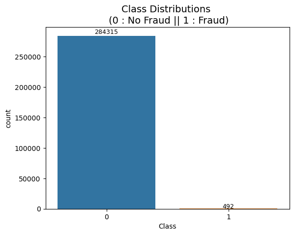
데이터 분리
- 데이터의 불균형이 매우 크므로 stratify 옵션 필수!!
- stratify : 학습과 테스트 데이터 동일 비율 설정
from sklearn.model_selection import train_test_split

X = raw_data.iloc[:, 1:-1]  # Featueres Data
y = raw_data.iloc[:, -1]    # Labels Data

print('Data Shape : ', X.shape, y.shape)
X_train, X_test, y_train, y_test = train_test_split(X, y, test_size=0.3, random_state=13, stratify=y)
------------------------------------
Data Shape :  (284807, 29) (284807,)
데이터 비율 확인
import numpy as np

print('Fraud Data Ratio of "y_train": ', np.unique(y_train, return_counts=True)[1][1] / len(y_train) * 100, '%')
------------------------------------------------------
Fraud Data Ratio of "y_train":  0.17254870488152324 %
1st Trial
Classifier score return function
from sklearn.metrics import accuracy_score, precision_score, recall_score, f1_score, roc_auc_score

def get_clf_eval(y_test, pred):
    acc = accuracy_score(y_test, pred)
    pre = precision_score(y_test, pred)
    re = recall_score(y_test, pred)
    f1 = f1_score(y_test, pred)
    auc = roc_auc_score(y_test, pred)

    return acc, pre, re, f1, auc
Confusion_matrix return function
from sklearn.metrics import confusion_matrix

def print_clf_eval(y_test, pred):
    confusion = confusion_matrix(y_test, pred)
    acc, pre, re, f1, auc = get_clf_eval(y_test, pred)

    print('=> confusion matrix')
    print(confusion)
    print('======================')
    print(f'Accuacy: {acc:.4f}, Precision: {pre:.4f}')
    print(f'Recall: {re:.4f}, F1: {f1:.4f}, AUC: {auc:.4f}')
LogisticRegression
from sklearn.linear_model import LogisticRegression

lr_clf = LogisticRegression(random_state=13, solver='liblinear')
lr_clf.fit(X_train, y_train)
lr_pred = lr_clf.predict(X_test)

print('Logistic Regression')
print_clf_eval(y_test, lr_pred)
---------------------------------------
Logistic Regression
=> confusion matrix
[[85284    11]
 [   60    88]]
======================
Accuacy: 0.9992, Precision: 0.8889
Recall: 0.5946, F1: 0.7126, AUC: 0.7972
DecisionTree
from sklearn.tree import DecisionTreeClassifier

dt_clf = DecisionTreeClassifier(random_state=13, max_depth=4)
dt_clf.fit(X_train, y_train)
dt_pred = dt_clf.predict(X_test)

print('Decision Tree')
print_clf_eval(y_test, dt_pred)
------------------------------------------
Decision Tree
=> confusion matrix
[[85281    14]
 [   42   106]]
======================
Accuacy: 0.9993, Precision: 0.8833
Recall: 0.7162, F1: 0.7910, AUC: 0.8580
RandomForest
from sklearn.ensemble import RandomForestClassifier

rf_clf = RandomForestClassifier(random_state=13, n_jobs=6, n_estimators=100)
rf_clf.fit(X_train, y_train)
rf_pred = rf_clf.predict(X_test)

print('Random Forest')
print_clf_eval(y_test, rf_pred)
------------------------------------------
Random Forest
=> confusion matrix
[[85290     5]
 [   38   110]]
======================
Accuacy: 0.9995, Precision: 0.9565
Recall: 0.7432, F1: 0.8365, AUC: 0.8716
Light GBM
from lightgbm import LGBMClassifier

lgbm_clf = LGBMClassifier(n_estimators=1000, num_leaves=64, n_jobs=6, boost_from_average=False)
lgbm_clf.fit(X_train, y_train)
lgbm_pred = lgbm_clf.predict(X_test)

print('Light GBM')
print_clf_eval(y_test, lgbm_pred)
--------------------------------------------
Light GBM
=> confusion matrix
[[85289     6]
 [   34   114]]
======================
Accuacy: 0.9995, Precision: 0.9500
Recall: 0.7703, F1: 0.8507, AUC: 0.8851
주관적인 Recall과 Precision 해석
- 은행입장 : Recall이 높으면 좋을 것
    - 모든 범죄를 검거하고 싶음
- 사용자 입장 : Precision이 높으면 좋을 것
    - 정상 사용자가 의심 받을 수 있음(귀찮)
- 가장 좋은 것은 둘다 좋은 F1-Score가 높은 것
모델 입력시 성능 출력 함수
def get_result(model, X_train, y_train, X_test, y_test):
    model.fit(X_train, y_train)
    pred = model.predict(X_test)

    return get_clf_eval(y_test, pred)
다수의 모델의 성능을 정리해서 DF으로 반환하는 함수
def get_result_pd(models, model_names, X_train, y_train, X_test, y_test):
    col_names = ['accuracy', 'precision', 'recall', 'f1', 'roc_auc']
    tmp = []

    for model in models:
        tmp.append(get_result(model, X_train, y_train, X_test, y_test))

    return pd.DataFrame(tmp, columns=col_names, index=model_names)
4개의 분류 모델 성능 확인
- 정확도는 중요하지 않음(데이터의 비율상 모두 높게 출력됨)
- 앙상블 계열의 성능 우수(Recall)
import time

models = [lr_clf, dt_clf, rf_clf, lgbm_clf]
model_names = ['LogisticReg.', 'DecisionTree', 'RandomForest', 'LightGBM']

start_time = time.time()
results = get_result_pd(models, model_names, X_train, y_train, X_test, y_test)

print('Fit time : ', time.time() - start_time)
results
----------------------------------------------------------------
Fit time :  107.24186658859253

              accuracy  precision    recall        f1   roc_auc
LogisticReg.  0.999169   0.888889  0.594595  0.712551  0.797233
DecisionTree  0.999345   0.883333  0.716216  0.791045  0.858026
RandomForest  0.999497   0.956522  0.743243  0.836502  0.871592
LightGBM      0.999532   0.950000  0.770270  0.850746  0.885100
2nd Trial(데이터 정리)
'Amount' 분포 확인
- 대다수의 인원이 적은 금액을 사용함
- 소수의 인원이 많은 금액을 사용함
plt.figure(figsize=(10,5))
sns.distplot(raw_data['Amount'])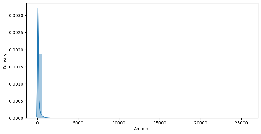
StandardScaler 적용
from sklearn.preprocessing import StandardScaler

scaler = StandardScaler()
amount_n = scaler.fit_transform(raw_data['Amount'].values.reshape(-1, 1))

raw_data_copy = raw_data.iloc[:, 1:-2]
raw_data_copy['Amount_Scaled'] = amount_n
raw_data_copy.head()
-------------------------------------------------------------------------------
         V1        V2        V3        V4        V5        V6        V7  \
0 -1.359807 -0.072781  2.536347  1.378155 -0.338321  0.462388  0.239599
1  1.191857  0.266151  0.166480  0.448154  0.060018 -0.082361 -0.078803
2 -1.358354 -1.340163  1.773209  0.379780 -0.503198  1.800499  0.791461
3 -0.966272 -0.185226  1.792993 -0.863291 -0.010309  1.247203  0.237609
4 -1.158233  0.877737  1.548718  0.403034 -0.407193  0.095921  0.592941

         V8        V9       V10  ...       V20       V21       V22       V23  \
0  0.098698  0.363787  0.090794  ...  0.251412 -0.018307  0.277838 -0.110474
1  0.085102 -0.255425 -0.166974  ... -0.069083 -0.225775 -0.638672  0.101288
2  0.247676 -1.514654  0.207643  ...  0.524980  0.247998  0.771679  0.909412
3  0.377436 -1.387024 -0.054952  ... -0.208038 -0.108300  0.005274 -0.190321
4 -0.270533  0.817739  0.753074  ...  0.408542 -0.009431  0.798278 -0.137458

        V24       V25       V26       V27       V28  Amount_Scaled
0  0.066928  0.128539 -0.189115  0.133558 -0.021053       0.244964
1 -0.339846  0.167170  0.125895 -0.008983  0.014724      -0.342475
2 -0.689281 -0.327642 -0.139097 -0.055353 -0.059752       1.160686
3 -1.175575  0.647376 -0.221929  0.062723  0.061458       0.140534
4  0.141267 -0.206010  0.502292  0.219422  0.215153      -0.073403

[5 rows x 29 columns]
모델 학습
X_train, X_test, y_train, y_test = train_test_split(X, y, test_size=0.3, random_state=13, stratify=y)

models = [lr_clf, dt_clf, rf_clf, lgbm_clf]
model_names = ['LogisticReg.', 'DecisionTree', 'RandomForest', 'LightGBM']

start_time = time.time()
results = get_result_pd(models, model_names, X_train, y_train, X_test, y_test)

print('Fit time : ', time.time() - start_time)
results
-----------------------------------------------------------------
Fit time :  101.21563196182251
              accuracy  precision    recall        f1   roc_auc
LogisticReg.  0.999169   0.888889  0.594595  0.712551  0.797233
DecisionTree  0.999345   0.883333  0.716216  0.791045  0.858026
RandomForest  0.999497   0.956522  0.743243  0.836502  0.871592
LightGBM      0.999532   0.950000  0.770270  0.850746  0.885100
ROC 커브
from sklearn.metrics import roc_curve

def draw_roc_curve(models, model_names, X_test, y_test):
    plt.figure(figsize=(10,10))

    for model in range(len(models)):
        pred = models[model].predict_proba(X_test)[:, 1]
        fpr, tpr, thresholds = roc_curve(y_test, pred)
        plt.plot(fpr, tpr, label=model_names[model])

    plt.plot([0,1],[0,1], 'k--', label='random quess')
    plt.title('ROC')
    plt.legend()
    plt.xlabel('FPR'); plt.ylabel('TPR')
    plt.grid()
    plt.show()

draw_roc_curve(models, model_names, X_test, y_test)
log scale
amount_log = np.log1p(raw_data['Amount'])

raw_data_copy['Amount_Scaled'] = amount_log
raw_data_copy.head()
-------------------------------------------------------------------------------
         V1        V2        V3        V4        V5        V6        V7  \
0 -1.359807 -0.072781  2.536347  1.378155 -0.338321  0.462388  0.239599
1  1.191857  0.266151  0.166480  0.448154  0.060018 -0.082361 -0.078803
2 -1.358354 -1.340163  1.773209  0.379780 -0.503198  1.800499  0.791461
3 -0.966272 -0.185226  1.792993 -0.863291 -0.010309  1.247203  0.237609
4 -1.158233  0.877737  1.548718  0.403034 -0.407193  0.095921  0.592941

         V8        V9       V10  ...       V20       V21       V22       V23  \
0  0.098698  0.363787  0.090794  ...  0.251412 -0.018307  0.277838 -0.110474
1  0.085102 -0.255425 -0.166974  ... -0.069083 -0.225775 -0.638672  0.101288
2  0.247676 -1.514654  0.207643  ...  0.524980  0.247998  0.771679  0.909412
3  0.377436 -1.387024 -0.054952  ... -0.208038 -0.108300  0.005274 -0.190321
4 -0.270533  0.817739  0.753074  ...  0.408542 -0.009431  0.798278 -0.137458

        V24       V25       V26       V27       V28  Amount_Scaled
0  0.066928  0.128539 -0.189115  0.133558 -0.021053       5.014760
1 -0.339846  0.167170  0.125895 -0.008983  0.014724       1.305626
2 -0.689281 -0.327642 -0.139097 -0.055353 -0.059752       5.939276
3 -1.175575  0.647376 -0.221929  0.062723  0.061458       4.824306
4  0.141267 -0.206010  0.502292  0.219422  0.215153       4.262539

[5 rows x 29 columns]
log_scale 분포 시각화
plt.figure(figsize=(10, 5))
sns.distplot(raw_data_copy['Amount_Scaled'], color='r')
모델 학습
- 결과에 큰 변화는 없음
X_train, X_test, y_train, y_test = train_test_split(raw_data_copy, y, test_size=0.3, random_state=13, stratify=y)

start_time = time.time()
results = get_result_pd(models, model_names, X_train, y_train, X_test, y_test)

print('Fit time : ', time.time() - start_time)
results
-----------------------------------------------------------------
Fit time :  94.71821999549866
              accuracy  precision    recall        f1   roc_auc
LogisticReg.  0.999157   0.887755  0.587838  0.707317  0.793854
DecisionTree  0.999345   0.883333  0.716216  0.791045  0.858026
RandomForest  0.999497   0.956522  0.743243  0.836502  0.871592
LightGBM      0.999532   0.950000  0.770270  0.850746  0.885100
ROC 커브
- 큰 변화는 없음
draw_roc_curve(models, model_names, X_test, y_test)
3rd Trial(Outlier 정리)
'V14' 칼럼에 이상치가 존재
sns.boxplot(data=raw_data[['V13', 'V14', 'V15']])
Outlier의 인덱스 반환 함수
def get_outlier(df=None, column=None, weight=1.5):
    fraud = df[df['Class']==1][column]
    quantile_25 = np.percentile(fraud.values, 25)
    quantile_75 = np.percentile(fraud.values, 75)

    iqr = quantile_75 - quantile_25
    iqr_weight = iqr * weight
    lowest_val = quantile_25 - iqr_weight
    highest_val = quantile_75 + iqr_weight

    outlier_index = fraud[(fraud < lowest_val) | (fraud > highest_val)].index

    return outlier_index
outlier 찾기
get_outlier(df=raw_data, column='V14', weight=1.5)
---------------------------------------------------
Int64Index([8296, 8615, 9035, 9252], dtype='int64')
outlier 제거
print('삭제 전 : ', raw_data_copy.shape)

outlier_index = get_outlier(df=raw_data, column='V14', weight=1.5)
raw_data_copy.drop(outlier_index, axis=0, inplace=True)
print('삭제 후 : ', raw_data_copy.shape)
-----------------------------------------
삭제 전 :  (284807, 29)
삭제 후 :  (284803, 29)
이상치 제거 후 모델 학습
- RandomForest
- recall : 0.7432 -> 0.7739 - LightGBM
- recall : 0.7702 -> 0.8082
X = raw_data_copy

raw_data.drop(outlier_index, axis=0, inplace=True)
y = raw_data.iloc[:, -1]

X_train, X_test, y_train, y_test = train_test_split(X, y, test_size=0.3, random_state=13, stratify=y)

start_time = time.time()
results = get_result_pd(models, model_names, X_train, y_train, X_test, y_test)

print('Fit time : ', time.time() - start_time)
results
draw_roc_curve(models, model_names, X_test, y_test)
----------------------------------------------------------------
Fit time :  122.6107828617096
              accuracy  precision    recall        f1   roc_auc
LogisticReg.  0.999286   0.904762  0.650685  0.756972  0.825284
DecisionTree  0.999427   0.870229  0.780822  0.823105  0.890311
RandomForest  0.999497   0.918699  0.773973  0.840149  0.886928
LightGBM      0.999602   0.951613  0.808219  0.874074  0.904074
ROC 커브
- 상당히 큰 변화
draw_roc_curve(models, model_names, X_test, y_test)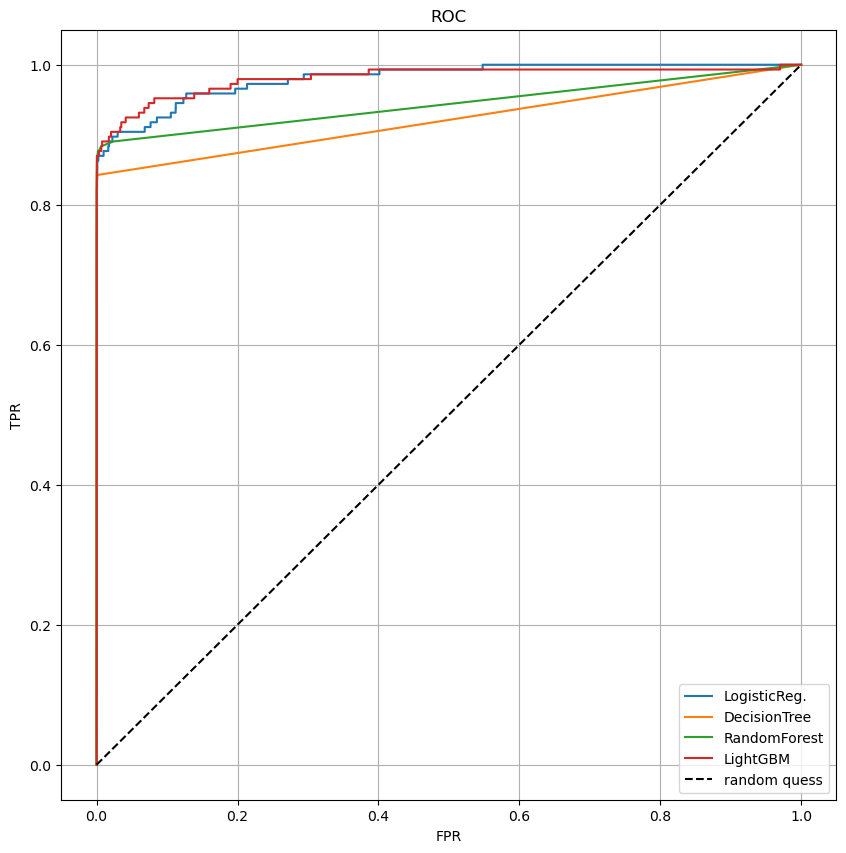
5) 4th Trial(SMOTE OverSampling)
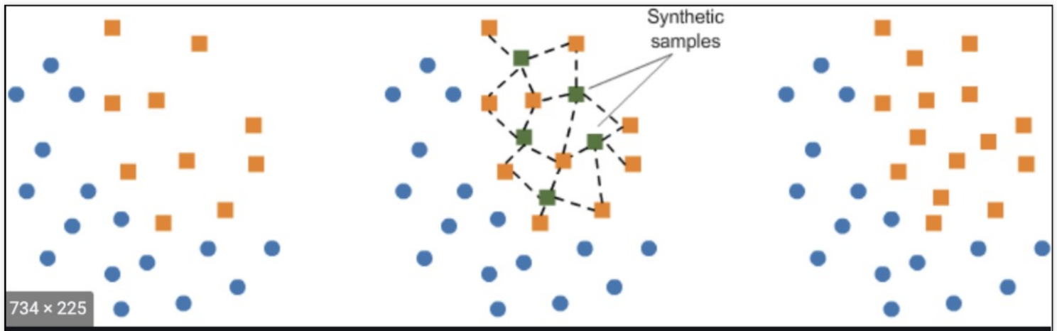
- 데이터의 불균형이 극심할 때 불균형한 두 클래스의 분포를 강제로 맞추는 작업
- 오버샘플링
- 원본데이터의 피처 값들을 변경하여 증식
- SMOTE(Synthetic Minority Over-sampliing Technique) 방법이 있음
- 적은 데이터 세트에 있는 개별 데이터를 *KNN방법으로 찾아서 데이터의 분포 사이에 새로운 데이터를 만드는 방식
- imbalanced-learn 활용
KNN(K-Nearest_Neighber)이란
새로운 데이터가 있을 때, K갯수에 해당하는 주변 데이터가 어느 그룹에 속하는지를 참고하여 새로운 데이터의 그룹을 결정하는 방법
SMOTE 적용
from imblearn.over_sampling import SMOTE

smote = SMOTE(random_state=13)
X_train_over, y_train_over = smote.fit_resample(X_train, y_train)
데이터 증강효과 비교
print('증강 전: ', np.unique(y_train, return_counts=True))
print('증강 후: ', np.unique(y_train_over, return_counts=True))
---------------------------------------------------------------------------------
증강 전:  (array([0, 1], dtype=int64), array([199020,    342], dtype=int64))
증강 후:  (array([0, 1], dtype=int64), array([199020, 199020], dtype=int64))
증강된 데이터로 모델 학습
- 전체적으로 극적인 성능변화 발생
- 특히 로지스틱회귀에 큰 변화
- recall : 0.6506 -> 0.8972
start_time = time.time()
results = get_result_pd(models, model_names, X_train_over, y_train_over, X_test, y_test)

print('Fit time : ', time.time() - start_time)
results
-----------------------------------------------------------------
Fit time :  219.28552627563477
              accuracy  precision    recall        f1   roc_auc
LogisticReg.  0.975609   0.059545  0.897260  0.111679  0.936502
DecisionTree  0.968984   0.046048  0.869863  0.087466  0.919509
RandomForest  0.999532   0.873239  0.849315  0.861111  0.924552
LightGBM      0.999532   0.873239  0.849315  0.861111  0.924552
ROC 커브
draw_roc_curve(models, model_names, X_test, y_test)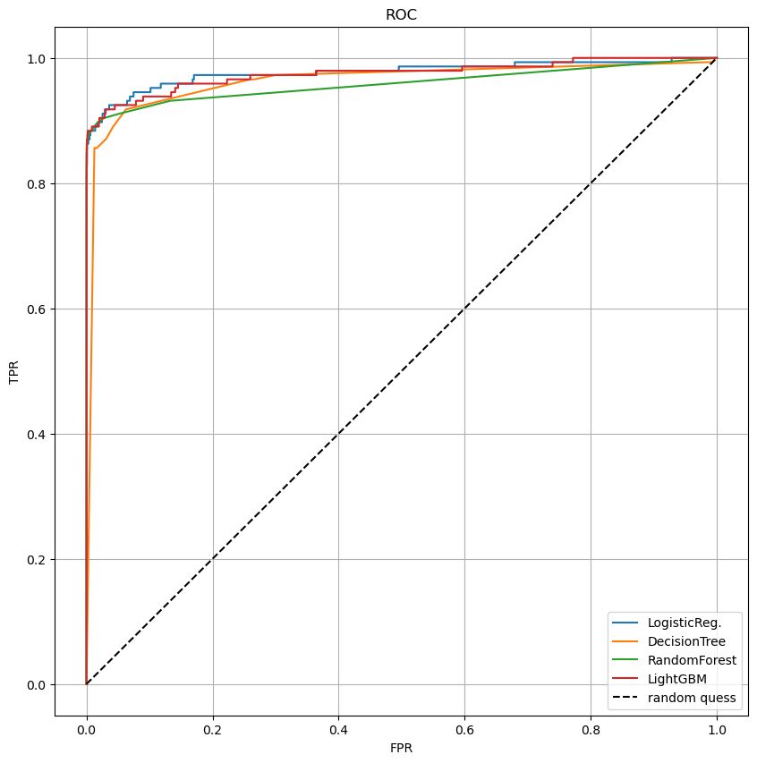
6) 학습내용 정리
- 매우 편향된 데이터 처리 실습
- 모델의 학습 및 평가 함수화
- recall과 precision의 의미
- SMOTE를 이용한 OverSampling