python -4. data preprocessing(3)

이상치처리
1. 이상치
📌 1. 이상치(outlier)
-
일부 관측치의 값이 전체 데이터의 범위에서 크게 벗어난 극단적인 값을 갖는 것
-
분산을 과도하게 증가시켜 검정력, 예측력 등 통계적 특성 약화시킴
-
전체 데이터 수가 많으면 이상치 영향이 감소함
-
통계적 이상치 발생 원인
- 입력 오류: 수집과정에서 발생하는 오류, 전체 데이터분포를 보고 쉽게 발견 가능
- 측정 오류: 데이터 입력 과정에서 발생하는 오류
- 실험 오류: 실험조건이 동일하지 않은 경우 발생하는 오류
- 고의적인 이상값: 자기 보고식 측정에서 나타나는 오류
- 표본 추출 오류: 데이터 샘플링(sampling)하는 과정에서 발생하는 오류
📌 2. 이상치 검출
1. 이상치 검출 방법
- 개별 데이터 관찰 : 전체 데이터의 추이나 특이사항 관찰하여 이상값 검출
- 통계 기법 사용: 통계 지표 데이터(평균, 중앙값, 최빈값)과 데이터 분산도를 활용해 이상치 검출
- 시각화 이용: 확률밀도함수, 히스토그램, 시계열 차트 등 활용
- 머신 러닝 기법 이용: 데이터 군집화를 통한 이상치 검출
📌 3. 단변량 이상치 검출 방법
- 정규분포(standard deviation)
데이터의 분포가 정규분포를 이룰 때, 데이터의표준편차를 이용해 이상치를 찾아내는 방법

📋 68-95-99.7 규칙(3시그마 규칙)
경험적인 규칙(empirical rule)이라고도 한다. 평균에서 양쪽으로 3표준편차의 범위에 거의 모든 값들(99.7%)이 들어간다.
-
1표준편차: 약 68%의 값들이 양쪽으로 1표준편차 범위(μ±σ)에 존재한다
-
2표준편차 : 약 95%의 값들이 평균에서 양쪽으로 2 표준편차 범위(μ±2σ)에 존재한다.
-
3표준편차 : 거의 모든 값들(실제로는 99.7%)이 평균에서 양쪽으로 3표준편차 범위(μ±3σ)에 존재한다.
데이터가 ±3σ 밖에 존재할 확률은 0.3%이기 때문에 이 범위를 벗어나는 값은 이상치로 간주
📋 z-score(표준화 점수) 이용
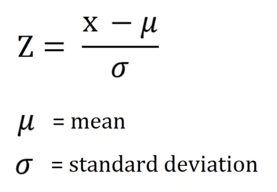
-
Z-score: 해당 데이터가 평균으로부터 얼마의 표준편차만큼 벗어나 있는가를 나타내는 지표
-
Z-score 가 3 보다 크고 -3 보다 작은 데이터를 이상치로 처리
- IQR(Interquantile Range, 사분위수) 이용
데이터의 분포가 정규분포를 이루지 않거나 한쪽으로 skewed된 경우 IQR값을 이용해 이상치 탐지
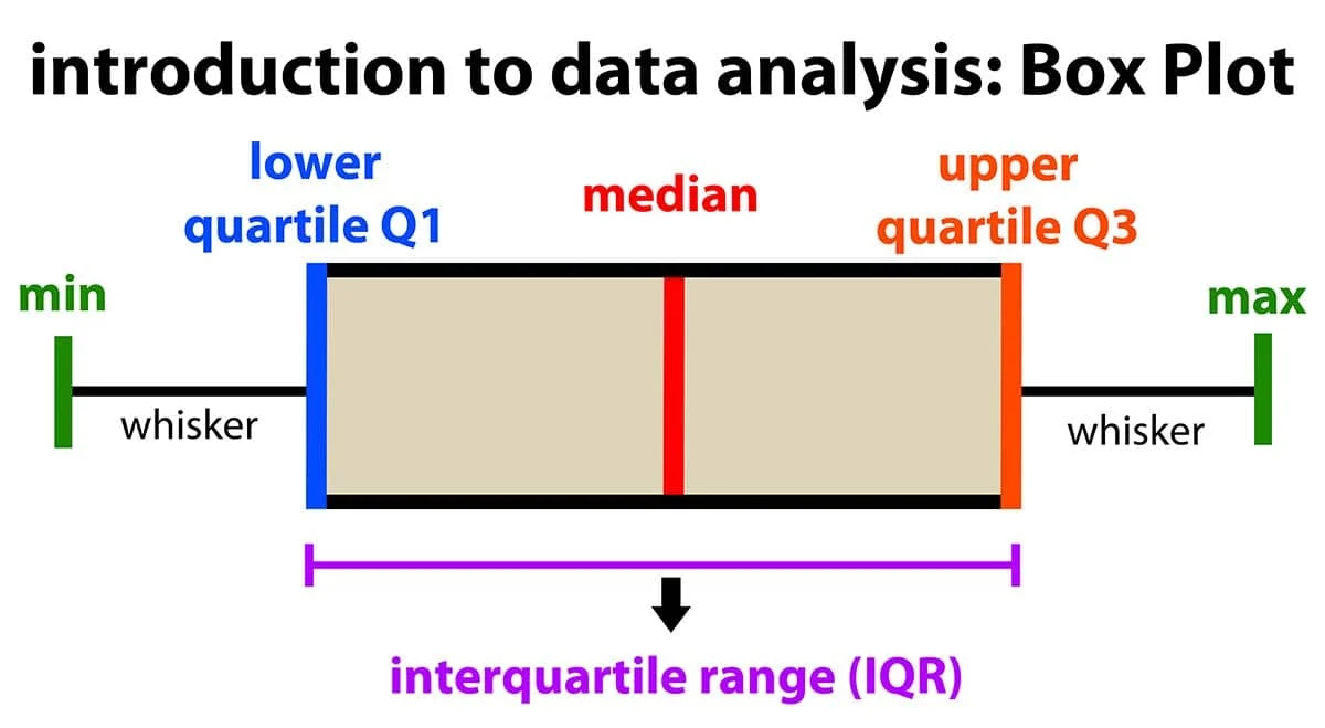
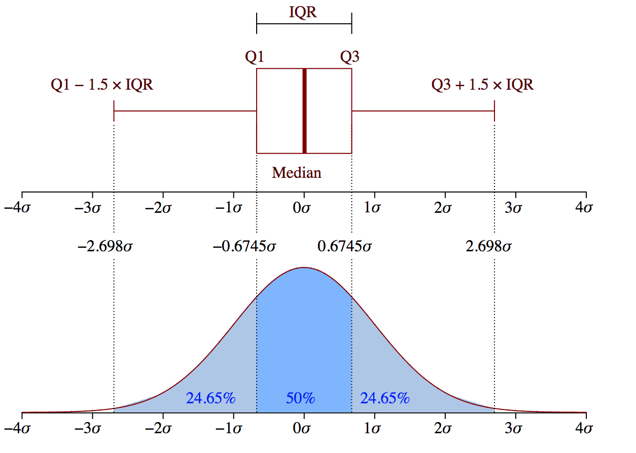
- (Q1-1.5IQR)보다 작거나 (Q3+1.5IQR)보다 큰 경우, 이상치로 간주
- Dixon's Q-test
모집단이 정규분포를 만족하는 단변량 자료에서 순서통계량을 이용하여 이상치 검증
- 가설: 귀무가설 H0(이상치가 없다), 대립가설 H1(이상치가 1개 있다)
- 데이터 수가 30개 미만인 경우 시행
- Grubb's Test
정규분포를 따르는 데이터에서 하나의 이상치를 발견할 수 있는 검정 방법
- 가설 : 귀무가설 H0(이상치가 하나도 없다.), 대립가설 H1(이상치가 하나 있다.)
- 직관적이고 구현이 간단하다는 장점이 존재하지만 한 번에 하나의 이상치만 발견 가능.

G가 위 그림을 만족한다면 귀무가설 H0을 기각한다.
- G-ESD(Generalized Extreme Studentized Deviation) Test
Grubb's Test가 한 번에 이상치를 하나밖에 찾지 못하는 단점 보완. 사전에 이상치의 개수를 r로 정해줌
-가설 : 귀무가설 H0(이상치가 하나도 없다.), 대립가설 H1(이상치가 최대 r개 있다.)
-총 r번의 반복과정을 거친다.
📌 4. 단변량 이상치 검출 python 실습
- scikit posthocs 설치
pip install scikit-posthocsimport warnings
#hide warnings
warnings.filterwarnings("ignore")필요한 모듈 import 하기
import pandas as pd

from scipy.stats import t, zscore
df = pd.DataFrame({'x':[4,5,6,8,12,3,5,9,8,2,8,23,5,6,8,15]})
#Z-score을 이용한 이상치 검출
z = zscore(df.x)
print('Z-score Outliers: ', df.x[(z<-3)|(z>3)].values)Z-score Outliers: [23]- IQR을 이용한 이상치 검출
#seaborn boxplot 이용
import seaborn as sns
sns.boxplot(df.x)

#pandas 이용하기
Q1 = df.x.quantile(0.25)
Q3 = df.x.quantile(0.75)
IQR = Q3 - Q1
ols = df.x[(df.x < (Q1 - 1.5 * IQR)) | (df.x > (Q3 + 1.5 * IQR))]
print("IQR Outliers 1: ", ols.values)

#scikit-posthocs 사용하기
import scikit_posthocs as sp
print("IQR Outliers 2: ", sp.outliers_iqr(df.x, ret = "outliers"))
IQR Outliers 1: [23 15]
IQR Outliers 2: [23 15]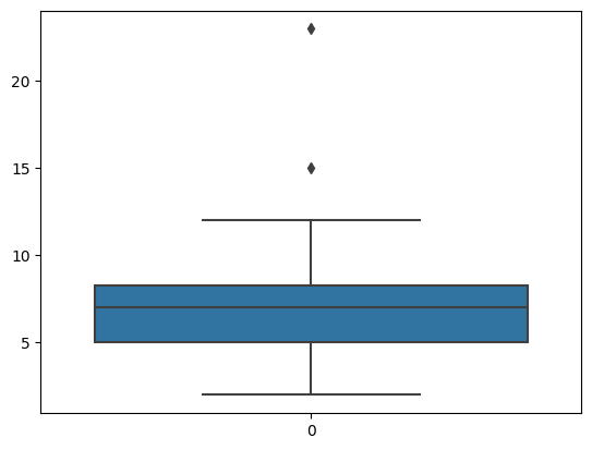
- Grubb's Test(ESD Test)
#scikit_posthocs 사용하기
import scikit_posthocs as sp

#outliers_grubbs는 inliers를 반환
inliers = sp.outliers_grubbs(df.x)
outliers = df.x[(df.x < inliers.min()) | (df.x > inliers.max())]

print("Grubbs Outliers: ", outliers.values)
Grubbs Outliers: [23]- Generalized ESD(G-ESD) Test
import scikit_posthocs as sp

#outliers_gesd는 test summary 제공
```python
print(sp.outliers_gesd(df.x, outliers = 3, report = True)) #이상치 개수 3개로 정한다.

inliers = sp.outliers_gesd(df.x)
outliers = df.x[(df.x < inliers.min()) | (df.x > inliers.max())]

print("G-ESD Outliers: ", outliers.values)
H0: no outliers in the data
Ha: up to 3 outliers in the data
Significance level: α = 0.05
Reject H0 if Ri > Critical Value (λi)
Summary Table for Two-Tailed Test
---------------------------------------
Exact Test Critical
Number of Statistic Value, λi
Outliers, i Value, Ri 5 %
---------------------------------------
1 2.906 2.586 *
2 2.379 2.548
3 2.13 2.507
G-ESD Outliers: [23]📌 5. 다변량 이상치 검출 방법
- 다변량 이상치 유형
- cross-trend outliers : 추세선에서 크게 벗어난 이상치, 원인 파악 어려움
- in-trend outliers : 추세선과 가깝지만 다른 데이터와 많이 떨어져있는 이상치, 일반적으로 원인 파악 용이
- Fringe Outliers : 추세선과 가까우나 별도의 추세를 가지는 것처럼 보이는 이상치, 일반적으로 원인 파악 어려움
- 회귀진단(regression diagnotics)
- 회귀계수 추정 후 잔차(residual)의 다양한 통계량을 사용하여 이상치 탐색, 회귀식 추정에 영향을 미치는 극단치를 탐색하는 것을 포함함
1) 레버리지(leverage)
- 독립변수의 각 관측치가 독립변수들의 평균에서 떨어진 정도를 반영하는 통계량
- 0과 1사이의 값을 가지며, 일반적으로 레버리지 평균의 2~4배를 초과하는 관측치를 이상치로 정의함
2) 표준화 잔차(standardized residual, Pearson residual)
- 표준화 잔차는 잔차를 표준화한 통계량임
- 일반적으로 표준화 잔차의 절대값이 2나 3을 초과하는 관측치를 이상치로 정의함
3) 스튜던트 잔차(studentized residual, internal)
- 잔차를 잔차의 표준오차로 나눈 통계량으로, t-분포를 기반으로
이상치를 탐색함 - 절대적인 수치로는 스튜던트 잔차의 절대값이 3 또는 4를 초과하면 이상치로 의심함
4) 쿡의 거리(Cook's distance)
- 추정된 회귀모형을 기반으로 이상치를 탐지함
- 추정된 회귀모형에 대한 각 관측치들의 전반적인 영향력 정도를 측정하기 위해 잔차와 레버리지를 동시에 고려한 척도임
- 쿡의 거리가 1보다 큰 경우, 강한 이상치로 판단함
5) DFFITS(Difference of fits)
- 모든 관측치를 활용하여 추정된 회귀모형의 예측치와 i번째 관측치를 제외한 후 추정된 회귀모형의 예측치 변화 정도를 측정하는 방법
- DFFITS 값이 클수록 이상치일 가능성이 높음
6) DFBETAS(Difference of betas)
- 모든 관측치를 활용하여 추정된 회귀모형의 회귀계수와 i번째 관측치를 제외한 후 추정된 회귀모형의 회귀계수 변화 정도를 측정하는 방법
- 데이터의 수가 적은 경우(n ≤ 30), DFBETAS의 절대값이 1보다 크면 이상치로 판단
- 데이터의 수가 큰 경우(n > 30), DFBEETAS의 절대값이 2/
sqrt(n)보다 클 경우 이상치로 판단
📌 6. 회귀진단 이상치 검출 python 실습
- statsmodels 패키지 사용
pip install statsmodels- 필요한 모듈 import 하기
import pandas as pd
import seaborn as sns
import sklearn
import statsmodels.api as sm
import statsmodels.formula.api as smf- sklearn의 diabetes 데이터셋 import
from sklearn.datasets import load_diabetes

temp = load_diabetes()
diabetes = pd.DataFrame(temp.data, columns = temp.feature_names)
diabetes['target'] = temp.target

diabetes.describe()
        age	             sex	         bmi	         bp	              s1	        s2	             s3	            s4	           s5	          s6   	          target
count	4.420000e+02	4.420000e+02	4.420000e+02	4.420000e+02	4.420000e+02	4.420000e+02	4.420000e+02	4.420000e+02	4.420000e+02	4.420000e+02	442.000000
mean	-2.511817e-19	1.230790e-17	-2.245564e-16	-4.797570e-17	-1.381499e-17	3.918434e-17	-5.777179e-18	-9.042540e-18	9.293722e-17	1.130318e-17	152.133484
std	4.761905e-02	4.761905e-02	4.761905e-02	4.761905e-02	4.761905e-02	4.761905e-02	4.761905e-02	4.761905e-02	4.761905e-02	4.761905e-02	77.093005
min	-1.072256e-01	-4.464164e-02	-9.027530e-02	-1.123988e-01	-1.267807e-01	-1.156131e-01	-1.023071e-01	-7.639450e-02	-1.260971e-01	-1.377672e-01	25.000000
25%	-3.729927e-02	-4.464164e-02	-3.422907e-02	-3.665608e-02	-3.424784e-02	-3.035840e-02	-3.511716e-02	-3.949338e-02	-3.324559e-02	-3.317903e-02	87.000000
50%	5.383060e-03	-4.464164e-02	-7.283766e-03	-5.670422e-03	-4.320866e-03	-3.819065e-03	-6.584468e-03	-2.592262e-03	-1.947171e-03	-1.077698e-03	140.500000
75%	3.807591e-02	5.068012e-02	3.124802e-02	3.564379e-02	2.835801e-02	2.984439e-02	2.931150e-02	3.430886e-02	3.243232e-02	2.791705e-02	211.500000
max	1.107267e-01	5.068012e-02	1.705552e-01	1.320436e-01	1.539137e-01	1.987880e-01	1.811791e-01	1.852344e-01	1.335973e-01	1.356118e-01	346.000000
필요한 column만 추출하기
diabetes_df = diabetes[['target', 'bmi', 'age', 'bp', 's1']]
diabetes_df.head()

diabetes_df.describe()
target bmi age bp s1
count 442.000000 4.420000e+02 4.420000e+02 4.420000e+02 4.420000e+02
mean 152.133484 -2.245564e-16 -2.511817e-19 -4.797570e-17 -1.381499e-17
std 77.093005 4.761905e-02 4.761905e-02 4.761905e-02 4.761905e-02
min 25.000000 -9.027530e-02 -1.072256e-01 -1.123988e-01 -1.267807e-01
25% 87.000000 -3.422907e-02 -3.729927e-02 -3.665608e-02 -3.424784e-02
50% 140.500000 -7.283766e-03 5.383060e-03 -5.670422e-03 -4.320866e-03
75% 211.500000 3.124802e-02 3.807591e-02 3.564379e-02 2.835801e-02
max 346.000000 1.705552e-01 1.107267e-01 1.320436e-01 1.539137e-01필요한 행 개수만큼 뽑아내기
diabetes_df2 = diabetes_df.loc[:50]
diabetes_df2.tail()
    target	bmi	         age	     bp	         s1
46	190.0	-0.011595	-0.056370	-0.033213	-0.046975
47	142.0	-0.073030	-0.078165	-0.057313	-0.084126
48	75.0	-0.041774	0.067136	0.011544	0.002559
49	142.0	0.014272	-0.041840	-0.005670	-0.012577
50	155.0	-0.007284	0.034443	0.014987	-0.044223
그래프로 확인하기
sns.pairplot(diabetes_df2, diag_kind='kde', hue='target')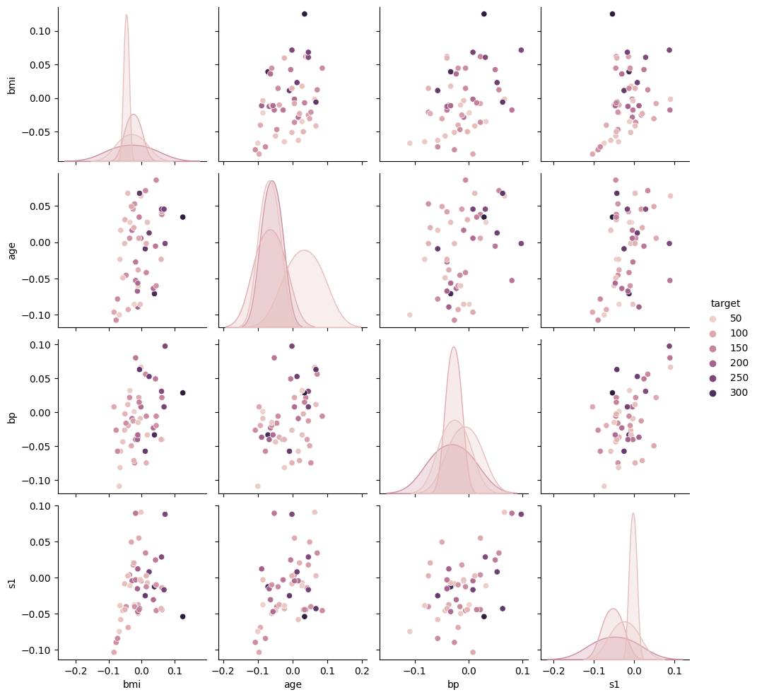
target과 bp(평균혈압), s1(혈중 총콜레스테롤), bmi(체질량지수) 회귀분석
lm = smf.ols(formula = 'target ~ bp  + s1 + bmi', data=diabetes_df2).fit()
print(lm.summary())
OLS Regression Results
==============================================================================
Dep. Variable: target R-squared: 0.359
Model: OLS Adj. R-squared: 0.318
Method: Least Squares F-statistic: 8.779
Date: Wed, 25 Oct 2023 Prob (F-statistic): 9.93e-05
Time: 08:34:38 Log-Likelihood: -279.86
No. Observations: 51 AIC: 567.7
Df Residuals: 47 BIC: 575.5
Df Model: 3
Covariance Type: nonrobust
==============================================================================
coef std err t P>|t| [0.025 0.975]
------------------------------------------------------------------------------
Intercept 146.5244 9.086 16.126 0.000 128.245 164.804
bp 385.1453 232.215 1.659 0.104 -82.010 852.301
s1 -279.1809 233.448 -1.196 0.238 -748.818 190.456
bmi 864.6318 206.623 4.185 0.000 448.961 1280.303
==============================================================================
Omnibus: 1.211 Durbin-Watson: 2.025
Prob(Omnibus): 0.546 Jarque-Bera (JB): 1.245
Skew: 0.318 Prob(JB): 0.537
Kurtosis: 2.573 Cond. No. 32.7
==============================================================================
Notes:
[1] Standard Errors assume that the covariance matrix of the errors is correctly specified.그래프로 확인하기
sns.regplot(data = diabetes_df2, x = 'bmi', y = 'target')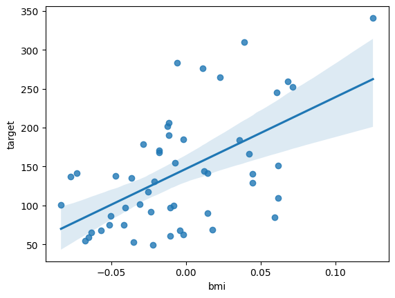
#d영향점 계산
import numpy as np
infl = lm.get_influence()

#레버리지 계산
leverage = infl.hat_matrix_diag
print('Leverage: \n', leverage)
print('Outliers using Leverage: \n', np.where(leverage > 3*np.mean(leverage)))
print()

#표준화 잔차 계산
resid_standard = lm.resid_pearson
print('Standardized Residuals: \n', resid_standard)
print('Outliers using Standardized Residuals: \n', np.where(np.abs(resid_standard) > 2))
print()
Leverage:
[0.10354066 0.04662681 0.06788243 0.0501539 0.05255526 0.06161349
0.04186991 0.16489683 0.0971582 0.05679002 0.21154607 0.03921261
0.02898369 0.02332454 0.04396454 0.19532752 0.06437108 0.07091656
0.02844567 0.03954563 0.0496828 0.03499839 0.02166552 0.0701661
0.04802844 0.03175364 0.12015131 0.10121174 0.06318353 0.13495096
0.05205642 0.08836085 0.26486851 0.05643238 0.06423789 0.14295632
0.06167685 0.05607036 0.18616497 0.10999851 0.08030518 0.12859542
0.03469098 0.11890871 0.07815716 0.06325184 0.03148321 0.09376109
0.04968295 0.02337951 0.05044304]
Outliers using Leverage:
(array([32]),)
Standardized Residuals:
[-1.14331373 -0.31582772 -0.89484224 1.42870186 0.20701763 -0.42867038
0.44692232 -1.35033281 -1.28583476 2.28175779 -0.08283343 -1.3436735
0.98038362 0.58754612 0.05568415 0.55888438 -0.4804774 -0.41266462
-0.60316198 0.84902622 -0.41568368 -1.46237901 -1.18756385 0.69137352
0.1117372 1.27396735 0.69716767 -1.79811657 0.33489004 1.73277183
-0.84080148 -0.17004347 0.98566634 -0.45047757 -0.34281892 0.24683756
1.32281619 2.21698036 0.50367656 -0.64761958 -0.53204758 -0.19492985
-1.38876006 -0.01907492 0.75120629 -1.28921215 0.87306277 0.93921139
-0.64253983 -0.29867054 -0.05491751]
Outliers using Standardized Residuals:
(array([ 9, 37]),)# 스튜던트 잔차 계산
resid_student = infl.resid_studentized_internal
print('Studentized Residuals: \n', resid_student)
print('Outliers using Studentized Residuals: \n', np.where(np.abs(resid_student) > 3))
print()
# 스튜턴트 제외 잔차 계산
resid_student_remove = infl.resid_studentized_external
print('Studentized Deleted Residuals: \n', resid_student_remove)
print('Outliers using Studentized Deleted Residuals: \n', np.where(np.abs(resid_student_remove) > 3))
print()Studentized Residuals:
[-1.20753609 -0.32345866 -0.92685357 1.46593592 0.21268183 -0.44251969
0.45658307 -1.4776472 -1.35325404 2.34944536 -0.09328622 -1.37081896
0.99490768 0.59452048 0.05695012 0.62303493 -0.49673087 -0.42812429
-0.61192813 0.86632877 -0.42641128 -1.4886614 -1.20064133 0.71698497
0.11452118 1.29468872 0.74324713 -1.89665853 0.3459991 1.863035
-0.8635793 -0.17809366 1.14960174 -0.46375292 -0.35439049 0.26663046
1.3655993 2.28187596 0.55832047 -0.68647481 -0.55478997 -0.20881824
-1.41349422 -0.02032133 0.78240348 -1.33202681 0.88713945 0.98660201
-0.65912198 -0.30222436 -0.05635732]
Outliers using Studentized Residuals:
(array([], dtype=int64),)
Studentized Deleted Residuals:
[-1.2135947 -0.32035588 -0.9254369 1.48459393 0.21050841 -0.43870159
0.45270479 -1.4970297 -1.36565009 2.47414036 -0.09229702 -1.38410921
0.99479784 0.59038592 0.05634295 0.61893244 -0.49271311 -0.42437359
-0.60780935 0.86398907 -0.42266897 -1.50873842 -1.20644544 0.71322769
0.11331213 1.30431117 0.73965738 -1.95258415 0.34273524 1.91518214
-0.86120275 -0.17624834 1.15364135 -0.45984616 -0.35106948 0.26397844
1.37862075 2.3939714 0.55418981 -0.68256312 -0.55066226 -0.20668072
-1.42908111 -0.02010408 0.77912581 -1.34338103 0.88509279 0.9863167
-0.65510709 -0.29928287 -0.05575643]
Outliers using Studentized Deleted Residuals:
(array([], dtype=int64),)# Cook's distance 계산
(cooks, p) = infl.cooks_distance
print('Cook\'s Distance: \n', cooks)
print('Outliers using Cook\'s Distance: \n', np.where(np.abs(cooks) > 1))
print()
# DFFITS 계산
(dffits, p) = infl.dffits_internal
print('DFFITS: \n', dffits)
print('Outliers using DFFITS: \n', np.where(dffits > 1))
print()
# DFBETAS 계산
dfbetas = infl.dfbetas
print('DFBETAS: \n', dfbetas)
print('Outliers using DFBETAS: \n', np.where(dfbetas.max(axis=1) > 1, ))
print()Cook's Distance:
[4.21037327e-02 1.27923514e-03 1.56404387e-02 2.83675221e-02
6.27282386e-04 3.21439497e-03 2.27749352e-03 1.07783853e-01
4.92681738e-02 8.30872483e-02 5.83718742e-04 1.91733793e-02
7.38639706e-03 2.11026242e-03 3.72870253e-05 2.35564098e-02
4.24394242e-03 3.49762059e-03 2.74087954e-03 7.72551149e-03
Outliers using Cook's Distance:
(array([], dtype=int64),)
DFFITS:
[-0.41038388 -0.07153279 -0.25012348 0.33685321 0.05009121 -0.11339127
0.09544618 -0.65660902 -0.4439287 0.57649718 -0.04832054 -0.27693594
0.1718883 0.09187519 0.01221262 0.30696195 -0.1302911 -0.11828137
-0.10470682 0.17578978 -0.09749839 -0.28350188 -0.17867106 0.19695683
0.02572309 0.23446024 0.27465879 -0.63646702 0.08985653 0.73584889
-0.20237093 -0.05544558 0.6900492 -0.11341339 -0.09285279 0.10889551
0.35011295 0.55614608 0.26703264 -0.24133629 -0.16393757 -0.08021789
-0.26795948 -0.00746532 0.22781731 -0.3461291 0.15994763 0.31734523
-0.15070763 -0.04676105 -0.01298944]
Outliers using DFFITS:
(array([], dtype=int64),)
DFBETAS:
[[-1.37361996e-01 -1.44406499e-01 2.54536725e-01 -2.72538616e-01]
[-4.47809068e-02 1.07688566e-02 -2.53725973e-02 4.78686347e-02]
[-9.58084606e-02 -2.37519004e-02 1.43286132e-01 -1.74066285e-01]
[ 2.33501098e-01 -2.14265027e-01 2.32225703e-01 -1.96343042e-02]
Outliers using DFBETAS:
(array([], dtype=int64),)영향점 통계량 summary
df_infl = infl.summary_frame()
df_infl.head()
dfb_Intercept	dfb_bp	dfb_s1	dfb_bmi	cooks_d	standard_resid	hat_diag	dffits_internal	student_resid	dffits
0	-0.137362	-0.144406	0.254537	-0.272539	0.042104	-1.207536	0.103541	-0.410384	-1.213595	-0.412443
1	-0.044781	0.010769	-0.025373	0.047869	0.001279	-0.323459	0.046627	-0.071533	-0.320356	-0.070847
2	-0.095808	-0.023752	0.143286	-0.174066	0.015640	-0.926854	0.067882	-0.250123	-0.925437	-0.249741
3	0.233501	-0.214265	0.232226	-0.019634	0.028368	1.465936	0.050154	0.336853	1.484594	0.341141
4	0.034560	0.025405	0.008127	-0.032160	0.000627	0.212682	0.052555	0.050091	0.210508	0.049579
boxplot으로 확인하기
sns.boxplot(df_infl, orient='h')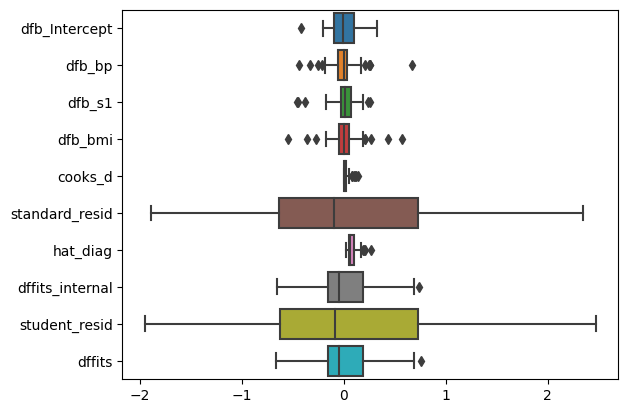
영향점(influence point) 그래프로 찾기
import matplotlib.pyplot as plt

fig, axs = plt.subplots(3, 2, figsize=(10, 10))
# 각 영향점 그래프
infl.plot_index(y_var="leverage", threshold=3*np.mean(leverage), ax=axs[0,0])
infl.plot_index(y_var="cooks", threshold=2*np.mean(cooks), ax=axs[0,1])
infl.plot_index(y_var="resid_student", threshold=1, ax=axs[1,0])
infl.plot_index(y_var="dfbeta", idx=1, threshold=0.5, ax=axs[1,1])

# 레버리지 vs. 스튜던트 잔차 플롯
sm.graphics.influence_plot(lm, criterion='cooks', ax=axs[2,0], plot_alpha=0.5)
sm.graphics.influence_plot(lm, criterion='DFFITS', ax=axs[2,1], plot_alpha=0.5)
fig.tight_layout()
plt.show()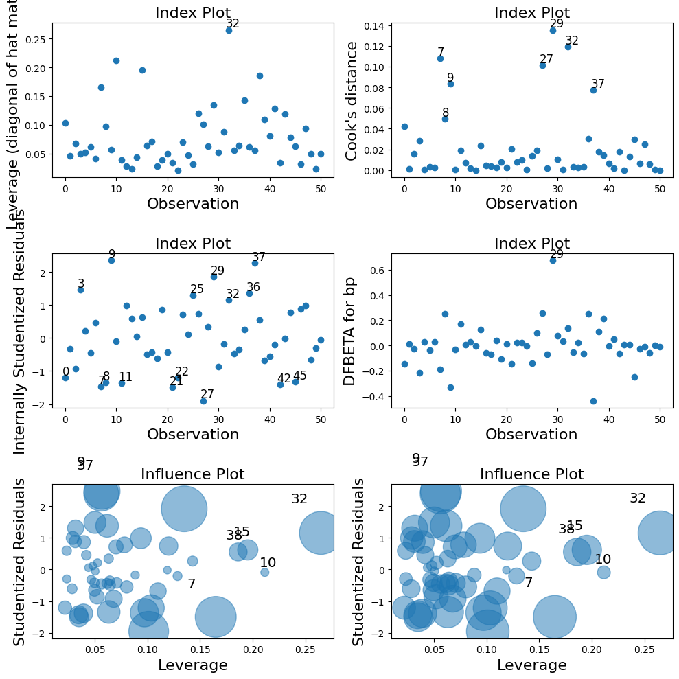
이상치들 제거한 후 회귀분석 재진행
# 이상치 제거한 후 회귀분석 실시
from sklearn.datasets import load_diabetes

temp = load_diabetes()
diabetes = pd.DataFrame(temp.data, columns = temp.feature_names)
diabetes['target'] = temp.target
diabetes_df = diabetes[['target', 'bmi', 'age', 'bp', 's1']]
diabetes_df = diabetes_df.loc[:50]
diabetes_df.drop([7, 8, 9,15, 27, 29, 32, 37, 38], inplace = True)


lm = smf.ols(formula = 'target ~ bp  + s1 + bmi', data=diabetes_df).fit()
print(lm.summary())
OLS Regression Results
==============================================================================
Dep. Variable: target R-squared: 0.325
Model: OLS Adj. R-squared: 0.271
Method: Least Squares F-statistic: 6.086
Date: Wed, 25 Oct 2023 Prob (F-statistic): 0.00174
Time: 08:47:36 Log-Likelihood: -220.89
No. Observations: 42 AIC: 449.8
Df Residuals: 38 BIC: 456.7
Df Model: 3
Covariance Type: nonrobust
==============================================================================
coef std err t P>|t| [0.025 0.975]
------------------------------------------------------------------------------
Intercept 140.6621 8.907 15.792 0.000 122.630 158.694
bp 258.9170 228.431 1.133 0.264 -203.518 721.352
s1 -92.7695 237.634 -0.390 0.698 -573.834 388.295
bmi 722.5574 229.612 3.147 0.003 257.732 1187.383
==============================================================================
Omnibus: 2.617 Durbin-Watson: 1.999
Prob(Omnibus): 0.270 Jarque-Bera (JB): 1.666
Skew: 0.245 Prob(JB): 0.435
Kurtosis: 2.156 Cond. No. 36.6
==============================================================================
Notes:
[1] Standard Errors assume that the covariance matrix of the errors is correctly specified.📌 7. 머신러닝을 통한 이상치 검출 python 실습
- scikit-learn 패키지 이용하기
import sklearn
from sklearn.datasets import load_diabetes
import pandas as pd- 데이터셋 로딩하기
temp = load_diabetes()
diabetes = pd.DataFrame(temp.data, columns = temp.feature_names)
diabetes['target'] = temp.target
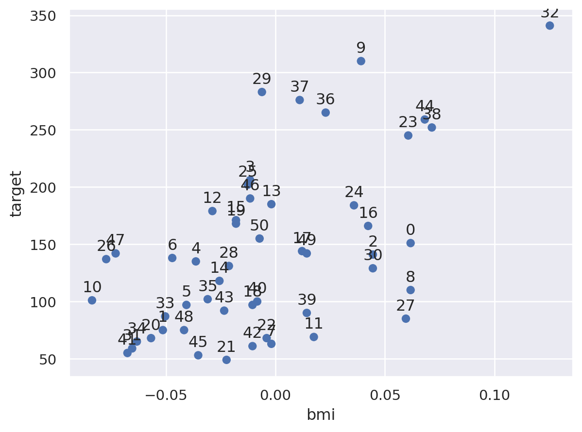
diabetes_df1 = diabetes[['target', 'bmi']]
diabetes_df2 = diabetes_df1.loc[:50]
import seaborn.objects as so
(
so.Plot(diabetes_df2, x = 'bmi', y = 'target', text = diabetes_df2.index)
.add(so.Dot())
.add(so.Text(valign = 'bottom'))
)
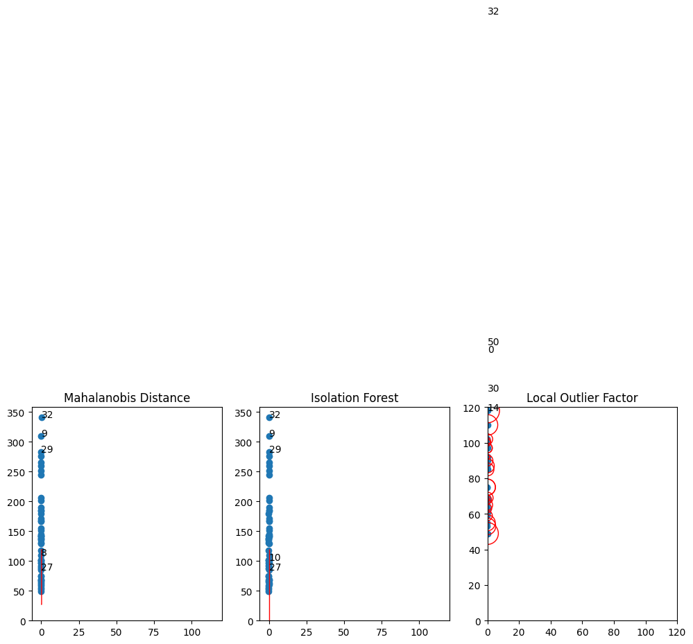
- MD, iForest, LOF 모형 학습시키기
from sklearn.covariance import EllipticEnvelope
from sklearn.ensemble import IsolationForest
from sklearn.neighbors import LocalOutlierFactor

#outliers 비중 초기값
outliers_fraction = 0.1

#모형의 인스턴스를 생성하고 데이터로 학습
md = EllipticEnvelope(contamination = outliers_fraction).fit(diabetes_df2)
iforest = IsolationForest(contamination = outliers_fraction).fit(diabetes_df2)

lof = LocalOutlierFactor(n_neighbors = 5, contamination = outliers_fraction)
import numpy as np
import matplotlib.pyplot as plt
import pandas as pd
#contour을 그리기 위한 데이터셋 생성
#meshgrid()를 이용해 바둑판 모양의 입력데이터 생성
xx, yy = np.meshgrid(np.linspace(0,120, 200), np.linspace(0,120,200))
df_test = pd.DataFrame(np.c_[xx.ravel(), yy.ravel()], columns=['bmi', 'target'])- 각각의 그래프 생성
#subplot 생성
fig, axs = plt.subplots(1, 3, figsize = (12, 4))

for i, method in enumerate([('Mahalanobis Distance', md), ('Isolation Forest', iforest)]):
  Z = method[1].predict(df_test).reshape(xx.shape)
  inliers = method[1].predict(diabetes_df2)
  print(f'{method[0]}:', inliers)
  axs[i].scatter(x=diabetes_df2['bmi'], y = diabetes_df2['target'])
  axs[i].contour(xx, yy, Z, levels=[0], linewidths=1, colors='red')
  for o, outlier in enumerate(inliers):
    if outlier == -1:
      axs[i].text(diabetes_df2['bmi'][o], diabetes_df2['target'][o], str(o))
    axs[i].set_title(method[0])


# Local Outlier Factor 그래프 출력
inliers = lof.fit_predict(diabetes_df2)
X_scores = lof.negative_outlier_factor_
print('Local Outlier Factor:', inliers)

axs[2].scatter(x=diabetes_df2['bmi'], y=diabetes_df2['target'])
# 데이터 포인트에 X_score의 크기에 따라 그려줄 반원 크기 계산
radius = (X_scores.max() - X_scores) / (X_scores.max() - X_scores.min())
axs[2].scatter(x=diabetes_df2['bmi'], y=diabetes_df2['target'], s=1000 * radius, edgecolors="r", facecolors="none")
for o, outlier in enumerate(inliers):
    if outlier == -1:
        axs[2].text(diabetes_df2['bmi'][o], diabetes_df2['target'][o],str(o))
axs[2].axis([0,120,0,120])
axs[2].set_title('Local Outlier Factor')

plt.show()
Mahalanobis Distance: [ 1 1 1 1 1 1 1 1 -1 -1 1 1 1 1 1 1 1 1 1 1 1 1 1 1
1 1 1 -1 1 -1 1 1 -1 1 1 1 1 1 1 1 1 1 1 1 1 1 1 1
1 1 1]
Isolation Forest: [ 1 1 1 1 1 1 1 1 1 -1 -1 1 1 1 1 1 1 1 1 1 1 1 1 1
1 1 1 -1 1 -1 1 1 -1 1 1 1 1 1 1 1 1 1 1 1 1 1 1 1
1 1 1]
Local Outlier Factor: [-1 1 1 1 1 1 1 1 1 1 1 1 1 1 -1 1 1 1 1 1 1 1 1 1
1 1 1 1 1 1 -1 1 -1 1 1 1 1 1 1 1 1 1 1 1 1 1 1 1
1 1 -1]