웹에서 가져오기(계속)

API 이용한 데이터 수집

#구글 맵스 설치
#pip install googlemaps
!pip install googlemaps
#메뉴 - 런타임- 런타임 다시 시작

#라이브러리 불러오기
import googlemaps
import pandas as pd

api_key = 'AIzaSyASvET9Cb7RaRwWe2kUklF3rqc90Ij2Bag'

# 구글 맵스 객체 생성
maps = googlemaps.Client(key = api_key)

maps.geocode("해운대해수욕장")[0].get('geometry')

{'location': {'lat': 35.1586975, 'lng': 129.1603842},
'location_type': 'APPROXIMATE',
'viewport': {'northeast': {'lat': 35.1600464802915, 'lng': 129.1617331802915},
'southwest': {'lat': 35.1573485197085, 'lng': 129.1590352197085}}}

# 장소 리스트를 이용하여 지오코딩하는 프로그램
places = ['해운대해수욕장','광안리해수욕장','송정해수욕장', '정동진역']
lat=[]
lng=[]
i = 0
for place in places:
  i +=2
  print(i, place)
  geo_coding = maps.geocode(place)[0].get('geometry')
  lat.append(geo_coding['location']['lat'])
  lng.append(geo_coding['location']['lat'])
df = pd.DataFrame({'위도': lat,
                   '경도': lng})
print(df)

2 해운대해수욕장
4 광안리해수욕장
6 송정해수욕장
8 정동진역
위도 경도
0 35.158698 35.158698
1 35.153170 35.153170
2 35.178613 35.178613
3 37.691884 37.691884

# 주소를 이용하여 지오코딩
maps.geocode("서울특별시 성동구 아차산로 111 2층")

[{'address_components': [{'long_name': '2층',
'short_name': '2층',
'types': ['subpremise']},
{'long_name': '111', 'short_name': '111', 'types': ['premise']},
{'long_name': 'Achasan-ro',
'short_name': 'Achasan-ro',
'types': ['political', 'sublocality', 'sublocality_level_4']},
{'long_name': 'Seongdong-gu',
'short_name': 'Seongdong-gu',
'types': ['political', 'sublocality', 'sublocality_level_1']},
{'long_name': 'Seoul',
'short_name': 'Seoul',
'types': ['administrative_area_level_1', 'political']},
{'long_name': 'South Korea',
'short_name': 'KR',
'types': ['country', 'political']},
{'long_name': '04794', 'short_name': '04794', 'types': ['postal_code']}],
'formatted_address': '2층, 111 Achasan-ro, Seongdong-gu, Seoul, South Korea',
'geometry': {'location': {'lat': 37.5448181, 'lng': 127.0565111},
'location_type': 'ROOFTOP',
'viewport': {'northeast': {'lat': 37.5461670802915,
'lng': 127.0578600802915},
'southwest': {'lat': 37.5434691197085, 'lng': 127.0551621197085}}},
'place_id': 'EjYy7Li1LCAxMTEgQWNoYXNhbi1ybywgU2Vvbmdkb25nLWd1LCBTZW91bCwgU291dGggS29yZWEiIBoeChYKFAoSCc_pXCuUpHw1EYcqPlP29I55EgQy7Li1',
'types': ['subpremise']}]

maps.geocode("서울특별시 성동구 아차산로 111 2층")[0].get('geometry')

{'location': {'lat': 37.5448181, 'lng': 127.0565111},
'location_type': 'ROOFTOP',
'viewport': {'northeast': {'lat': 37.5461670802915, 'lng': 127.0578600802915},
'southwest': {'lat': 37.5434691197085, 'lng': 127.0551621197085}}}

공공 데이터 포탈> 국토교통부, 아파트 머시기
한글 파일 다운로드>
api
서비스 url
응답 메시지 명세, 법정동, 아파트 이름,

데이터 살펴보기

데이터 프레임 구조

데이터 미리보기

https://archive.ics.uci.edu/ml/datasets/auto+mpg

#라이브러리 불러오기
import pandas as pd

# csv 파일 불러오기 + 열 이름이 없음(header = None)
df= pd.read_csv('/content/drive/MyDrive/hana1/Data/auto-mpg.csv', header = None)

# 열 이름
df.columns = ['mpg','cylinders','displacement','horsepower','weight',
              'acceleration','model_year','origin','car_name']

df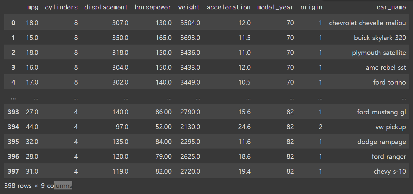

# 데이터 미리 보기 = 살펴복;
# head. tail
# 앞 부분 보기
df.head() # 기본값이 5개의 행

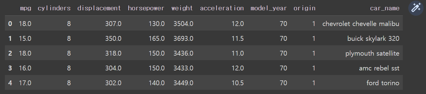
# 10개의 행
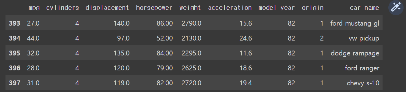
df.head(10)

# 뒷 부분 보기
df. tail() # 기본값이 5개의 행

데이터 요약 정보 확인

#데이터의 크기 확인 = 2개의 값이 튜플 형태로 풀력 = (행의 개수, 열의 개수)
df.shape 

(398, 9)

#데이터의 기본 정보
df.info() 
#DataFrame으로 저장됨, range index, 행 인덱스가 398개, (0~397), data columns열 9개 >>shape랑 똑같은 정보
#9개의 열 정보 알려줌
#object, 문자가 섞여있다

<class 'pandas.core.frame.DataFrame'>
RangeIndex: 398 entries, 0 to 397
Data columns (total 9 columns):

Column Non-Null Count Dtype

---

0 mpg 398 non-null float64
1 cylinders 398 non-null int64
2 displacement 398 non-null float64
3 horsepower 398 non-null object
4 weight 398 non-null float64
5 acceleration 398 non-null float64
6 model_year 398 non-null int64
7 origin 398 non-null int64
8 car_name 398 non-null object
dtypes: float64(4), int64(3), object(2)
memory usage: 28.1+ KB

# 데이터의 자료형 확인
# 데이터의 모든 열의 자료형
df.dtypes

mpg float64
cylinders int64
displacement float64
horsepower object
weight float64
acceleration float64
model_year int64
origin int64
car_name object
dtype: object

# 특정 열의 자료형
df.mpg.dtypes
df['mpg'].dtypes
df[['mpg','weight']].dtypes

dtype('float64')
dtype('float64')
mpg float64
weight float64
dtype: object

#기술통계 정보 요약
df.describe() # 요약할 수 있는 숫자형 열이 7개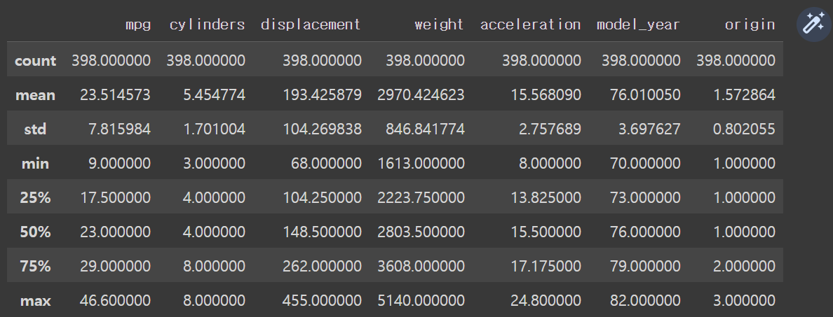

df.describe(include = 'all')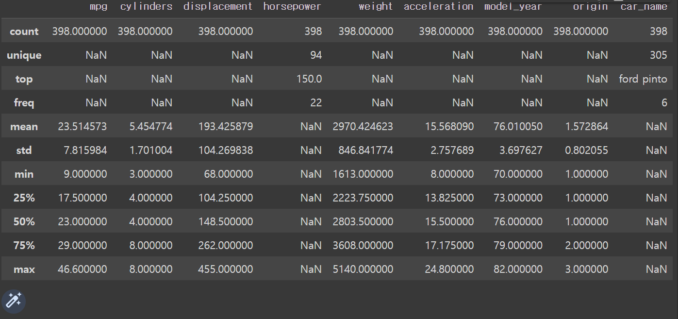

데이터 개수 확인

# 데이터의 모든 열의 개수 확인
print(df.count())
print(type(df.count()))

mpg 398
cylinders 398
displacement 398
horsepower 398
weight 398
acceleration 398
model_year 398
origin 398
car_name 398
dtype: int64
<class 'pandas.core.series.Series'>

# 특정 열의 개수 확인
print(df.mpg.count())
print(type(df.mpg.count()))
print(df['mpg'].count())
print(type(df['mpg'].count()))

398
<class 'numpy.int64'>
398
<class 'numpy.int64'>

print(df[['mpg','weight']].count())
print(type(df[['mpg','weight']].count()))

mpg 398
weight 398
dtype: int64
<class 'pandas.core.series.Series'>

#고유값 개수 = 빈도표 = 빈도가 높은 순으로 정렬
print(df.origin.value_counts())
print(type(df.origin.value_counts()))

1 249
3 79
2 70
Name: origin, dtype: int64
<class 'pandas.core.series.Series'>

print(df['origin'].value_counts())
print(type(df['origin'].value_counts()))

1 249
3 79
2 70
Name: origin, dtype: int64
<class 'pandas.core.series.Series'>

print(df[['origin','car_name']].value_counts())
print(type(df[['origin','car_name']].value_counts()))

origin car_name
1 ford pinto 6
ford maverick 5
amc matador 5
3 toyota corolla 5
1 chevrolet impala 4
..
ford ranger 1
ford thunderbird 1
ford torino 1
ford torino 500 1
3 toyouta corona mark ii (sw) 1
Length: 305, dtype: int64
<class 'pandas.core.series.Series'>

통계 함수

origin  car_name                   
1       ford pinto                     6
        ford maverick                  5
        amc matador                    5
3       toyota corolla                 5
1       chevrolet impala               4
                                      ..
        ford ranger                    1
        ford thunderbird               1
        ford torino                    1
        ford torino 500                1
3       toyouta corona mark ii (sw)    1
Length: 305, dtype: int64
<class 'pandas.core.series.Series'>

print(df[['mpg','weight']].mean())
print(type(df[['mpg','weight']].mean()))

mpg 23.514573
weight 2970.424623
dtype: float64
<class 'pandas.core.series.Series'>

# 중앙값
# 데이터 모든 열
print(df.median())
#특정 열
print(df.mpg.median())
print(df[['mpg','weight']].median())

mpg 23.0
cylinders 4.0
displacement 148.5
weight 2803.5
acceleration 15.5
model_year 76.0
origin 1.0
dtype: float64
23.0
mpg 23.0
weight 2803.5
dtype: float64
:3: FutureWarning: The default value of numeric_only in DataFrame.median is deprecated. In a future version, it will default to False. In addition, specifying 'numeric_only=None' is deprecated. Select only valid columns or specify the value of numeric_only to silence this warning.
print(df.median())

# 최댓값
# 데이터 모든 열
print(df.max())
#특정 열
print(df['mpg'].max())
print(df[['mpg','weight']].max())

mpg 46.6
cylinders 8
displacement 455.0
horsepower ?
weight 5140.0
acceleration 24.8
model_year 82
origin 3
car_name vw rabbit custom
dtype: object
46.6
mpg 46.6
weight 5140.0
dtype: float64

# 최소값
# 데이터 모든 열
print(df.min())
#특정 열
print(df['mpg'].median())
print(df[['mpg','weight']].min())
```python
mpg                                 9.0
cylinders                             3
displacement                       68.0
horsepower                        100.0
weight                           1613.0
acceleration                        8.0
model_year                           70
origin                                1
car_name        amc ambassador brougham
dtype: object
23.0
mpg          9.0
weight    1613.0
dtype: float64

# 표준편차
# 데이터 모든 열
print(df.std())
#특정 열
print(df['mpg'].std())
print(df[['mpg','weight']].std())

# 표준편차의 제곱 = 분산
# 표준편차 = 제곱근(분산)
print(df.mpg.std()**2)
print(df.mpg.var())

#분산
#데이터 모든 열
print(df.var())
#특정 열
print(df.mpg.var())
print(df['mpg'].var())
print(df[['mpg','weight']].var())

#상관계수
#상관행렬
print(df.corr())
print(df[['mpg', 'weight']].corr())
# 방향은 반대고, 크기는 크다

판다스 내장 그래프 도구

# 라이브러리 불러오기
import pandas as pd

#파일 경로, 파일 ㅣㅇ름, 파이 ㄹ확장자
#engine = None 기본값
df = pd.read_excel('/content/drive/MyDrive/hana1/Data/남북한발전전력량.xlsx', engine = 'openpyxl')

df.head(10)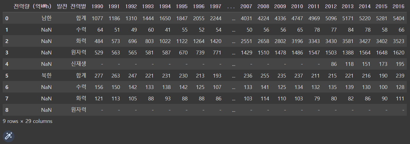

#남한, 1990-2016
df_new = df.iloc[[0,5],2:]
df_new.head()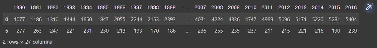

df_new.index = ["South", "North"]
df_new.head()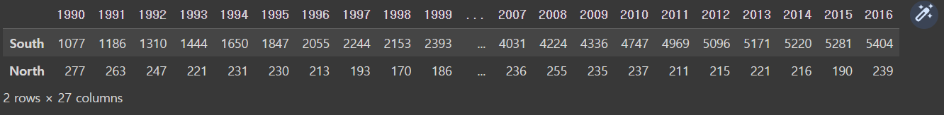

선 그래프

# 기본값 kind = 'line'
df_new.plot()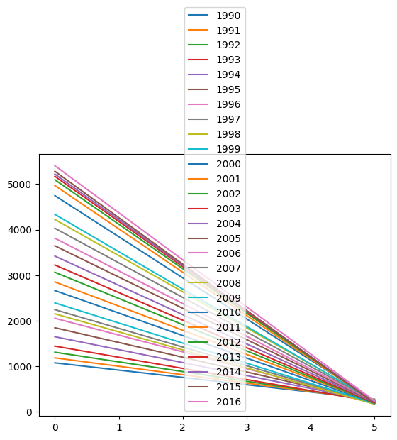

df_new_t = df_new.T
df_new_t.head()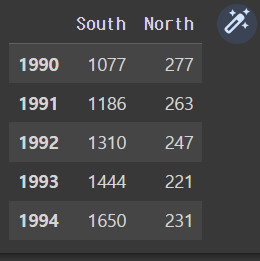

df_new_t.plot()
# = df_new_t.plot(kind = 'line')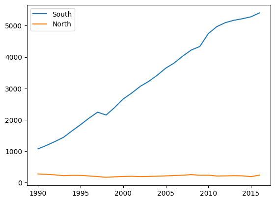

막대 그래프

#수직 막대 그래프
df_new.plot(kind ='bar')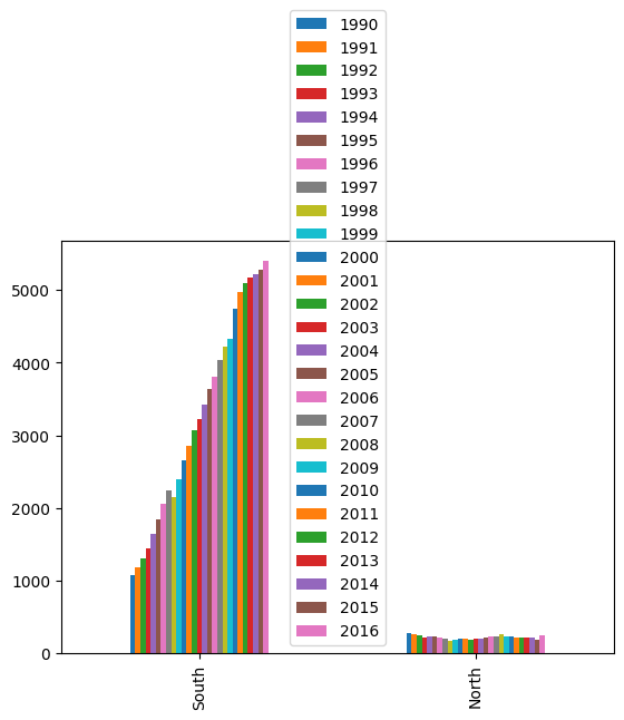

df_new_t.plot(kind = 'bar')
#kind = 'line'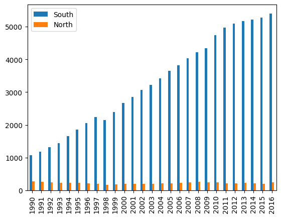

#수평 막대 그래프 
df_new_t.plot(kind='barh')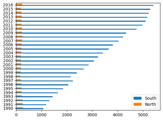

히스토그램

df_new_c = df_new_t.astype(int)
df_new_c.plot(kind ='hist')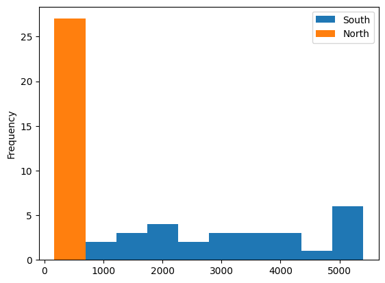

산점도

# csv 파일 불러오기 + 열 이름이 없음(header = None)
df= pd.read_csv('/content/drive/MyDrive/hana1/Data/auto-mpg.csv', header = None)
#열 이름 지정
df.columns = ['mpg','cylinders','displacement','horsepower','weight',
              'acceleration','model_year','origin','car_name']
df.head()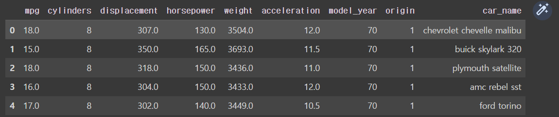

# 치중과 연비의 산점도
df.plot(kind = 'scatter', x = 'mpg', y = 'weight')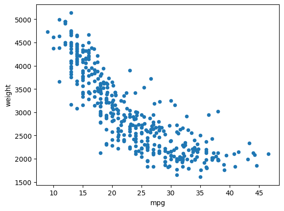

상자수염그림

https://ko.wikipedia.org/wiki/%EC%83%81%EC%9E%90_%EC%88%98%EC%97%BC_%EA%B7%B8%EB%A6%BC

• 1) 백분위 수 : 데이터를 백등분 한 것
• 2) 사분위 수 : 데이터를 4등분 한 것
• 3) 중위수 : 데이터의 정 가운데 순위에 해당하는 값.(관측치의 절반은 크거나 같고 나머지 절반은 작거나 같다.)
• 4) 제 3사분위 수 (Q3) : 중앙값 기준으로 상위 50% 중의 중앙값, 전체 데이터 중 상위 25%에 해당하는 값
• 5) 제 1사분위 수 (Q1) : 중앙값 기준으로 하위 50% 중의 중앙값, 전체 데이터 중 하위 25%에 해당하는 값
• 6) 사분위 범위 수(IQR) : 데이터의 중간 50% (Q3 - Q1)

  df[['mpg','acceleration']].plot(kind = 'box')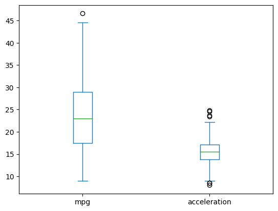

1QR 2분위 수
요정도는 정상범위야
데이터 기반으로 정하면(?) 이상치 발견할 수 있다

시각화 도구

# 한글 폰트 설치
!sudo apt-get install -y fonts-nanum
!sudo fc-cache -fv
!rm ~/.cache/matplotlib -rf
# 메뉴 ~ 런타임 ~ 런타임 다시 시작

matplotlib

#라이브러리 불러오기
import pandas as pd
import matplotlib.pyplot as plt

#데이터 불러오기
df = pd.read_excel('/content/drive/MyDrive/hana1/Data/시도별 전출입 인구수.xlsx',
              engine = 'openpyxl')
df.head()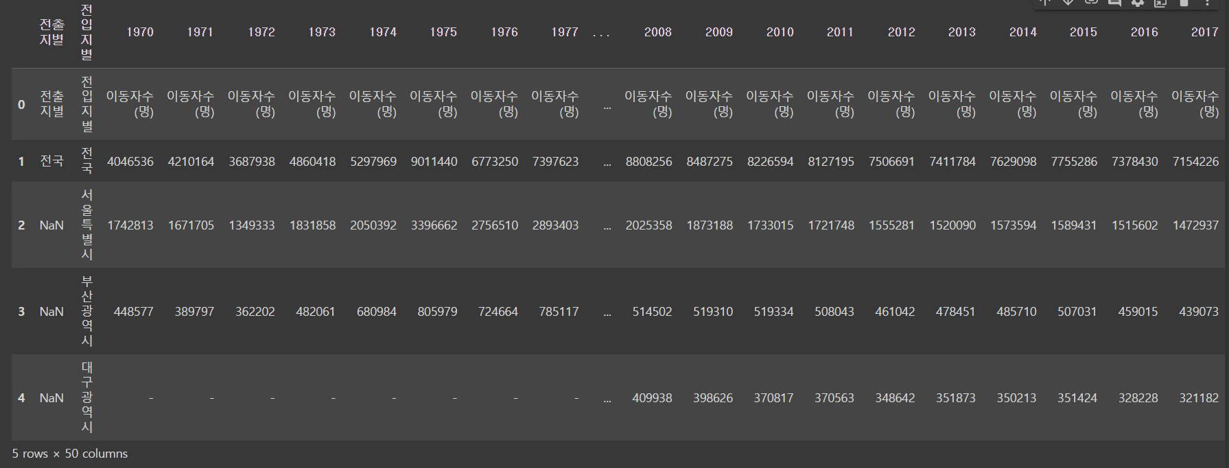

# Nan 값 채우기
df = df.fillna(method = 'ffill')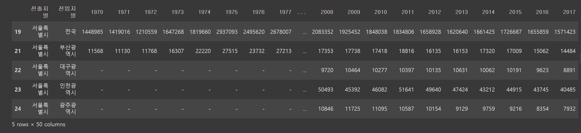

#전출지별 열 삭제
df_seoul = df_seoul.drop('전출지별', axis =1)
df_seoul.head()
#지우는 방향이 axis=1이야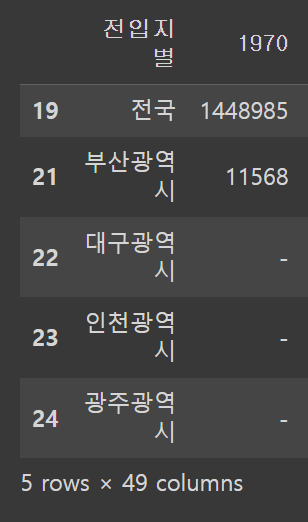

#열 이름 변경
df_seoul = df_seoul.rename({'전입지별':'전입지'}, axis = 1)
df_seoul.head()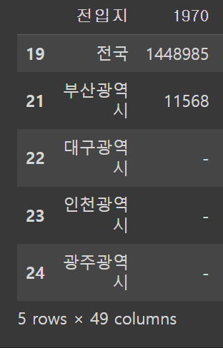

#행 인덱스 변경
df_seoul = df_seoul.set_index('전입지')
df_seoul.head()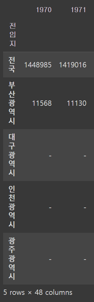

df_ggd = df_seoul.loc['경기도']
df_ggd
# 시리즈> 인덱스:값

1970 130149
1971 150313
1972 93333
1973 143234
1974 149045
1975 253705
1976 202276
1977 207722
1978 237684
1979 278411
1980 297539
1981 252073
1982 320174
...
2013 340801
2014 332785
2015 359337
2016 370760
2017 342433
Name: 경기도, dtype: object

선 그래프

plt.plot(df_ggd.index, df_ggd.values)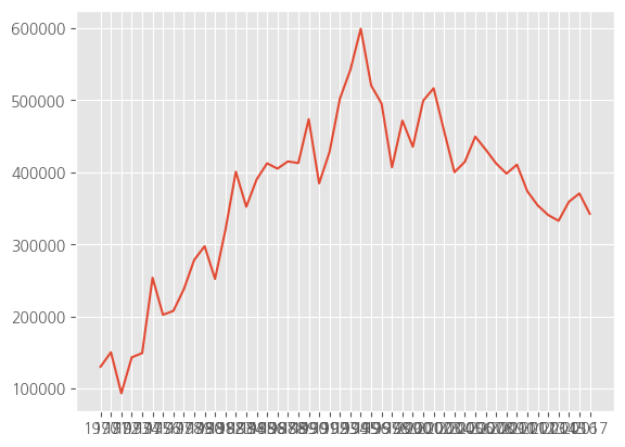

# 시리즈 데이터를 넣고 시각화해도 결과는 동일함
plt.plot(df_ggd)

차트 제목, 축 제목 추가

# 한글 폰트 지정
plt.rc("font", family ="NanumGothic")
# 선 그래프
plt.plot(df_ggd.index, df_ggd.values)
# 차트 제목 추가
plt.title("서울시에서 경기도로 이동하는 인구")
# 축 제목 추가
plt.xlabel("기간(연도)")
plt.ylabel("이동 인구 수")
plt.show()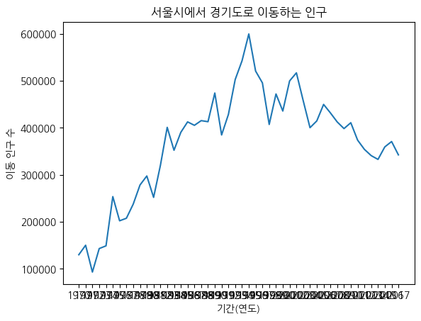

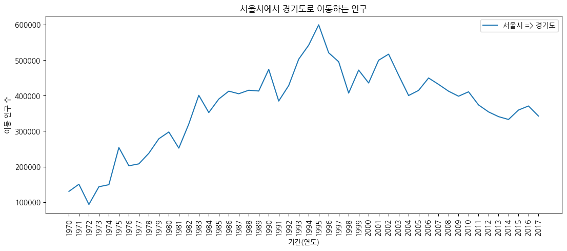
그래프 꾸미기

# 그림 사이즈 지정(가로, 세로)
plt.figure(figsize = (13,5))
# x 축 눈금 라벨 회전
plt.xticks(rotation = 'vertical')
# 선 그래프
plt.plot(df_ggd.index, df_ggd.values)
# 차트 제목 추가
plt.title("서울시에서 경기도로 이동하는 인구")
# 축 제목 추가
plt.xlabel("기간(연도)")
plt.ylabel("이동 인구 수")
# 범례 추가
plt.legend(labels = ["서울시 => 경기도"], loc = 'best')
plt.show()

  # 그래프 꾸미기
# 그림 사이즈 지정(가로, 세로)
plt.figure(figsize = (13,5))
# x 축 눈금 라벨 회전
plt.xticks(rotation = 'vertical')
# 선 그래프
plt.plot(df_ggd.index, df_ggd.values)
# 차트 제목 추가
plt.title("서울시에서 경기도로 이동하는 인구")
# 축 제목 추가
plt.xlabel("기간(연도)")
plt.ylabel("이동 인구 수")
# 범례 추가
plt.legend(labels = ["서울시 => 경기도"], loc = 'best')
plt.show()
  

스타일 서식

# 스타일 서식 확인
plt.style.available
#'ggplot',R에서 시각화하는 패키지, 파이썬에서 흉내냄
#'tableau-colorblind10']

['Solarize_Light2',
'_classic_test_patch',
'_mpl-gallery',
'_mpl-gallery-nogrid',
'bmh',
'classic',
'dark_background',
'fast',
'fivethirtyeight',
'ggplot',
'grayscale',
'seaborn-v0_8',
'seaborn-v0_8-bright',
'seaborn-v0_8-colorblind',
'seaborn-v0_8-dark',
'seaborn-v0_8-dark-palette',
'seaborn-v0_8-darkgrid',
'seaborn-v0_8-deep',
'seaborn-v0_8-muted',
'seaborn-v0_8-notebook',
'seaborn-v0_8-paper',
'seaborn-v0_8-pastel',
'seaborn-v0_8-poster',
'seaborn-v0_8-talk',
'seaborn-v0_8-ticks',
'seaborn-v0_8-white',
'seaborn-v0_8-whitegrid',
'tableau-colorblind10']

# 스타일 서식
plt.style.use('ggplot')
# 그림 사이즈 지정(가로, 세로)
plt.figure(figsize = (13, 5))
# x 축 눈금 라벨 회전
plt.xticks(rotation = 'vertical')
# 선 그래프
plt.plot(df_ggd.index, df_ggd.values)
# 차트 제목 추가
plt.title("서울시에서 경기도로 이동하는 인구")
# 축 제목 추가
plt.xlabel("기간(연도)")
plt.ylabel("이동 인구 수")
# 범례 추가
plt.legend(labels = ["서울시 => 경기도"], loc = 'best')
plt.show()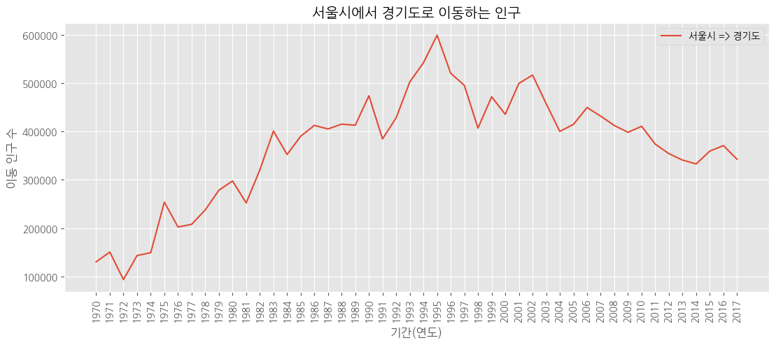

주석 추가

# 스타일 서식
plt.style.use('ggplot')
# 그림 사이즈 지정(가로, 세로)
plt.figure(figsize = (13, 5))
# x 축 눈금 라벨 회전
plt.xticks(rotation = 'vertical')
# 선 그래프
plt.plot(df_ggd.index, df_ggd.values)
# 차트 제목 추가
plt.title("서울시에서 경기도로 이동하는 인구")
# 축 제목 추가
plt.xlabel("기간(연도)")
plt.ylabel("이동 인구 수")
# 범례 추가
plt.legend(labels = ["서울시 => 경기도"], loc = 'best', fontsize = 15)
# y 축 범위 조정
plt.ylim(50000, 800000)
# 주석 추가
# 화살표
plt.annotate("", xy = (23, 620000), # 화살표 머리
           xytext = (3, 250000), # 화살표 꼬리
           xycoords = 'data', # 좌표계
           arrowprops = dict(arrowstyle = '->', color = 'red', lw = 10))
plt.annotate("", xy = (45, 400000), # 화살표 머리
           xytext = (29, 620000), # 화살표 꼬리
           xycoords = 'data', # 좌표계
           arrowprops = dict(arrowstyle = '->', color = 'blue', lw = 10))
# 텍스트
plt.annotate("인구 이동 증가",
           xy = (12, 400000), # 텍스트 시작 위치
           rotation = 25, # 회전
           va = 'baseline', # 위아래 정렬
           ha = 'center', # 좌우 정렬
           fontsize = 15)
plt.annotate("인구 이동 감소",
           xy = (37, 500000), # 텍스트 시작 위치
           rotation = -18, # 회전
           va = 'baseline', # 위아래 정렬
           ha = 'center', # 좌우 정렬
           fontsize = 15)
plt.show()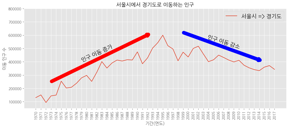

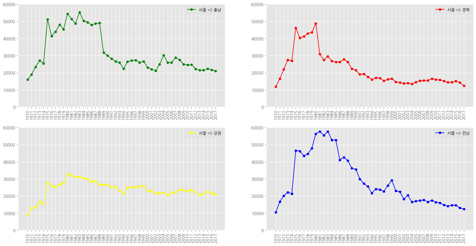
화면 분할

df_4 = df_seoul.loc[['충청남도','경상북도','강원도','전라남도']]
df_4.head()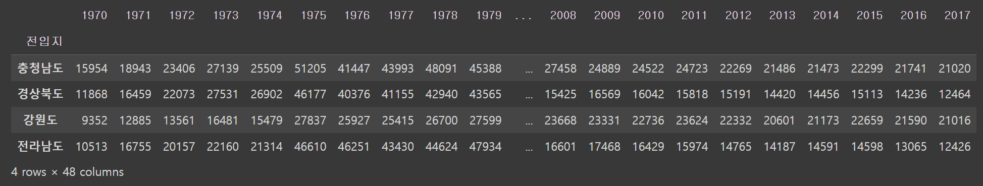

# 1970 ~ 2018 숫자 리스트
list(range(1970,2018))

# 연도 리스트 생성
# 1970 ~ 2018 문자열 리스트
col_years = list(map(str, range(1970,2018)))
col_years

# 한글 폰트 지정
plt.rc("font", family = "NanumGothic")
# 스타일 서식
plt.style.use('ggplot')
# 그래프 객체 만들기
fig = plt.figure(figsize = (20, 10))
ax1 = fig.add_subplot(2, 2, 1) # 행의 개수, 열의 개수, 위치
ax2 = fig.add_subplot(2, 2, 2)
ax3 = fig.add_subplot(2, 2, 3)
ax4 = fig.add_subplot(2, 2, 4)
# axe 객체에 그래프 추가
ax1.plot(col_years, df_4.loc['충청남도', :],  marker = 'o', markerfacecolor = 'green',
       markersize = 5, color = 'green', label = "서울 => 충남")
ax2.plot(col_years, df_4.loc['경상북도', :],  marker = 'o', markerfacecolor = 'red',
       markersize = 5, color = 'red', label = "서울 => 경북")
ax3.plot(col_years, df_4.loc['강원도', :],  marker = 'o', markerfacecolor = 'yellow',
       markersize = 5, color = 'yellow', label = "서울 => 강원")
ax4.plot(col_years, df_4.loc['전라남도', :],  marker = 'o', markerfacecolor = 'blue',
       markersize = 5, color = 'blue', label = "서울 => 전남")
# 범례 추가
ax1.legend(loc = 'best')
ax2.legend(loc = 'best')
ax3.legend(loc = 'best')
ax4.legend(loc = 'best')
# x 축 눈금 라벨 회전
ax1.set_xticklabels(col_years, rotation = 90)
ax2.set_xticklabels(col_years, rotation = 90)
ax3.set_xticklabels(col_years, rotation = 90)
ax4.set_xticklabels(col_years, rotation = 90)
# y 축 범위 조정
ax1.set_ylim(0, 60000)
ax2.set_ylim(0, 60000)
ax3.set_ylim(0, 60000)
ax4.set_ylim(0, 60000)
plt.show()