Lecture 2.1 - Traditional Feature-based Methods: Node

Traditional ML Pipeline

• Desgin features for nodes/links/graphs
• Obtain features for all training data
  
• Structural feature에 집중해서 알아본다. Network의 주변에 무엇이 있는지, 전체적인 graph의 특징은 무엇인지..
  Train an ML model
• Random forest
• SVM
• Neural network, etc
  Apply the model
• Given a new node/link/graph, obtain its features and make a prediction

This Lecture: Feature Design

• Using effective features over graphs is the key to achieving good test performance.
• Traditional ML pipeline uses hand-designed features
• In this lecture, we overview the traditional features for:

1. Node-level prediction
2. Link-level prediction
3. Graph-level prediction

• For simplicity, we focus on undirected graphs.

Machine Leraning in Graphs

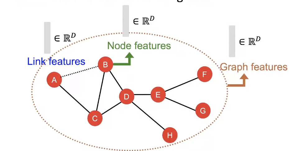
• Goal : Make predictions for a set of objects
• Design choices
  Features : d-dimensional vectors
  Objects : Nodes, edges, sets of nodes, entire graphs
  Objective function : What task are we aiming to solve?
  
• 해당 함수를 어떻게 학습시킬것인가????

Node-level Tasks

• Node classification → ML needs features
• Goal : Characterize the structure and position of a node in the network: node degree, node centrality, clustering coefficient, graphlets

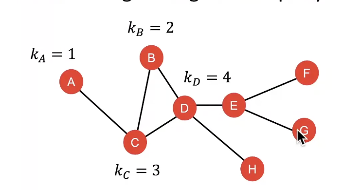
Node Degree

• The degre k_v of node v is the number of edges (neighboring nodes) the node has.
• Treats all neighboring nodes equally
  

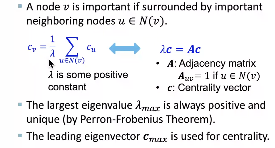
Node Centrality

• Node degree counts the neighboring nodes without capturing their importance.
• Node centrality c_v takes the node importance in a graph into account
• Engienvector centrality, Betweenness centrality, Closeness centrality, etc..

Eigenvector centrality

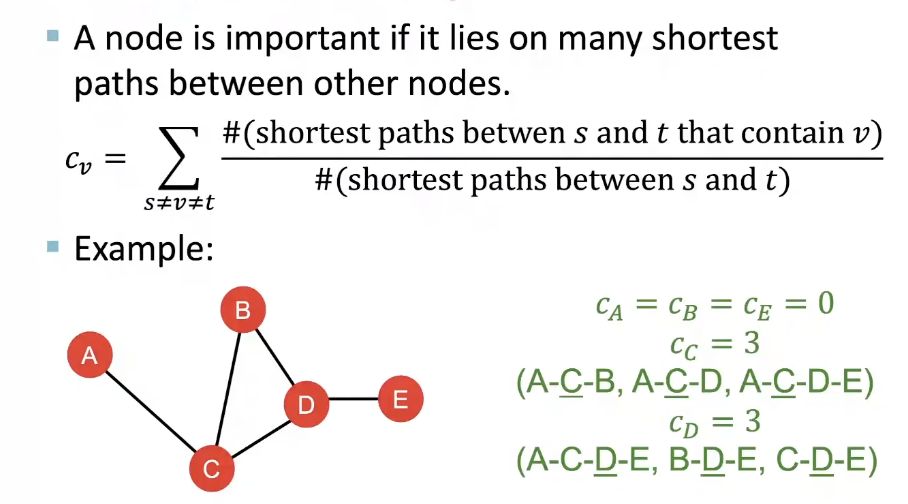
Betweenness centrality

Closeness centrality

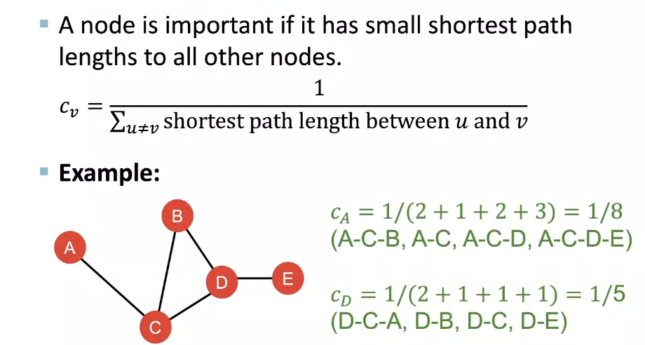
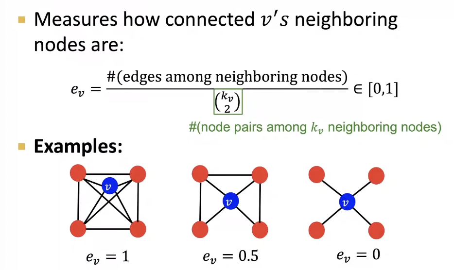
Clustering Coefficient

• 어떻게 주변 노드들과 연결되어 있는가?
  

Graphlets

• Observation : Clustering coefficient counts the #(triangles) in the ego-network
  
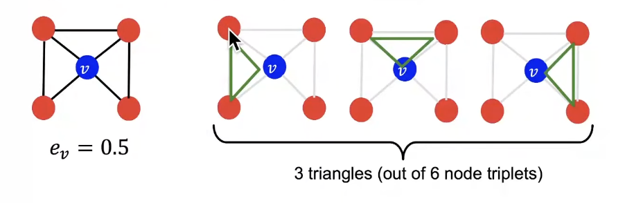
• We can generalize the above by counting #(pre-specified subgraphs, i.e., graphlets)
• Rooted connected non-isomorphic subgraphs
  
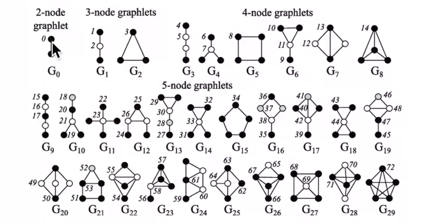
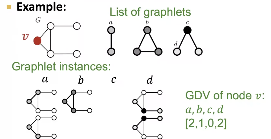
• Graphlet Degree Vector (GDV) : Graphlet-base features for nodes, A count vector of graphlets rooted at a given node!
• Degree count #(edges) that a node touches
• Clustering coefficient counts #(triangles) that a node touches.
• GDV counts #(graphlets) that a node touches
  
• Considering graphlets on 2 to 5 nodes we get:
  Vector of 73 coordinates is a signature of a node that describes the topology of node's neighborhood
  Captures its interconnectivities out to a distance of 4 hops
• Graphlet degree vector provides a measure of a node's local network topology
  Comparing vectors of two nodes provides a more detailed measure of local topological similarity than node degrees or clustering coefficient.

Lecture 2.2 - Traditional Feature-based Methods: Link

Link Prediction as a Task

Two formulations of the link prediction task
1. Links missing at random:
Remove a random set of links and them aim to predict them
2. Links over time: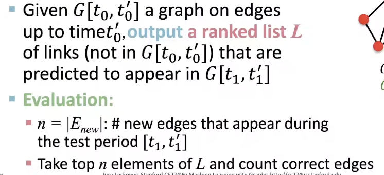

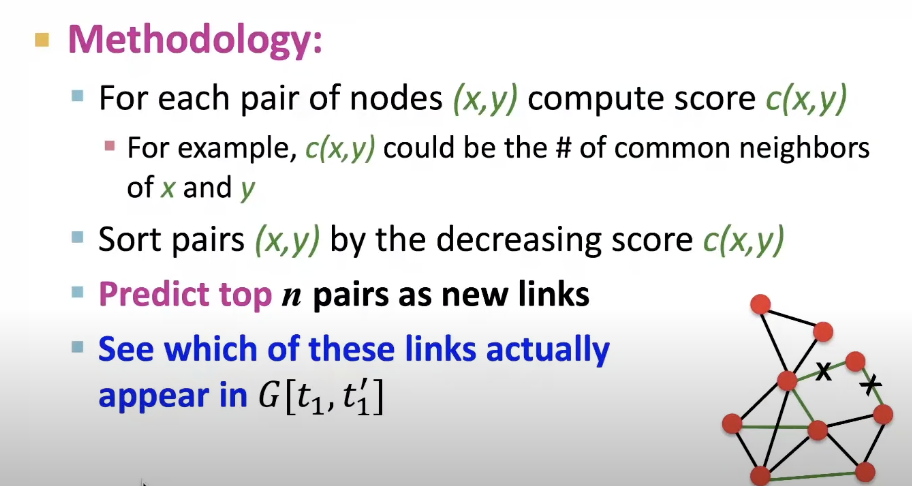
Link Prediction via Proximity

Link-Level Features

Distance-based feature

Shortest-path distance between two nodes

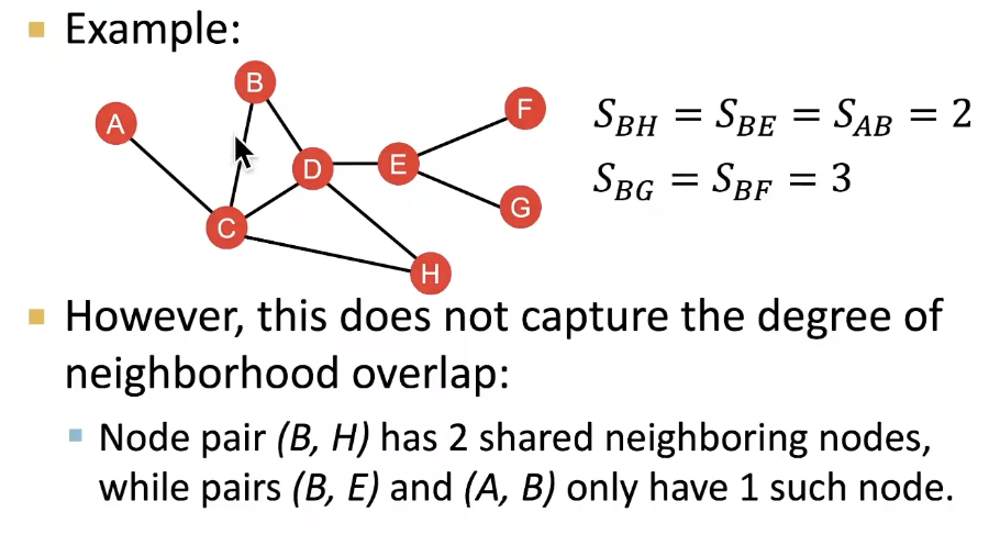
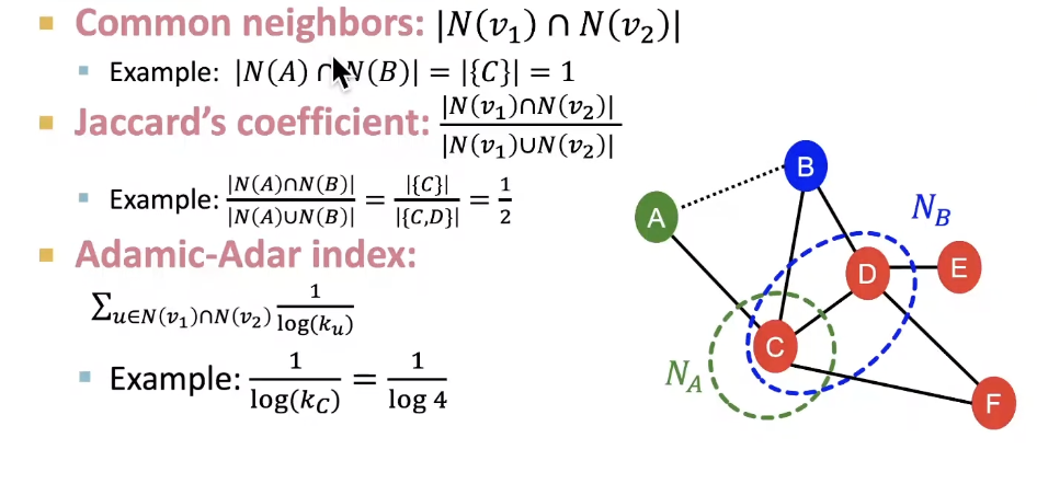
Local Neighborhood Overlap

Captures # neighboring nodes shared between two nodes v1 and v2

Global Neighborhood Overlap

• Limitaion of Local neighborhood features: Metric is always zero if the two nodes do not have any neighbors in common
• However, the two nodes may still potentially be connected in the future
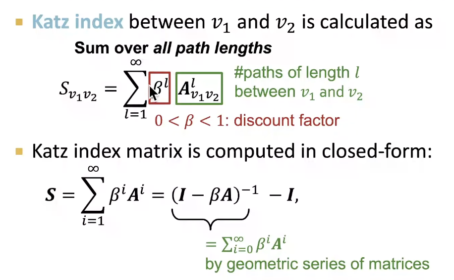
• Global neighborhood overlap metrics resolve the limitation by considering the entire graph.
• Katz index: count the number of paths of all lengths between given pair of nodes
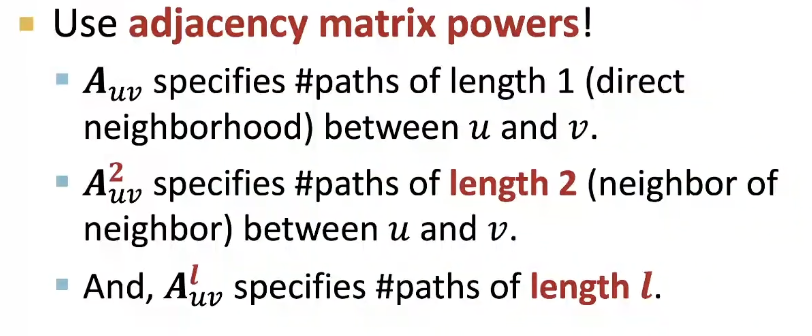
  Powers of adjacency matrix
  
  
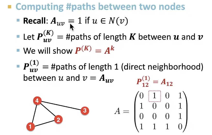
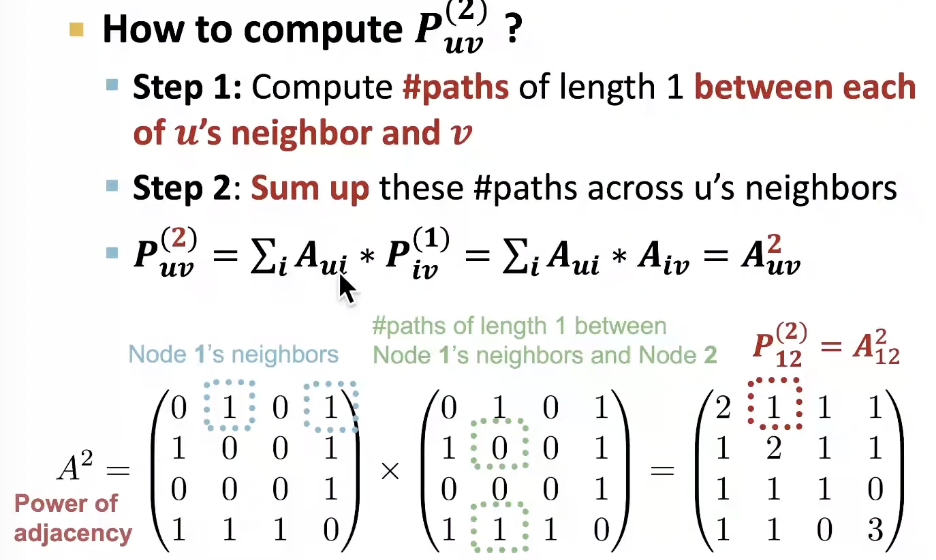
• How to compute # paths between two nodes?
  
  

Lecture 2.3 - Traditional Feature-based Methods: Graph

Graph-Level Features

• Goal : We want features that characterize the structure of an entire graph

Background: Kernel Methods

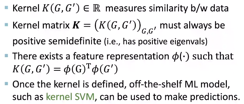
• Idea: Design Kernels instead of feature vectors.
• Graph Kernels: Measure similarity betwen two graphs:
  Graphlet Kernel, Wisfeiler-Lehman Kernel

Graph Kernel: Key Idea

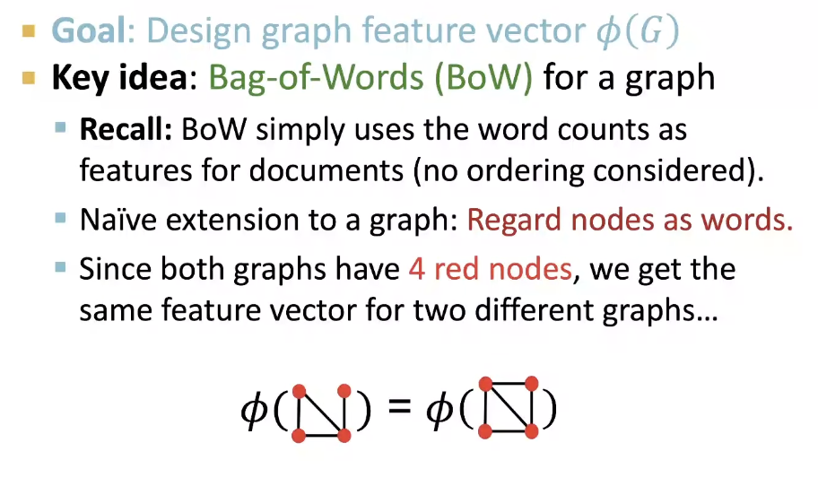
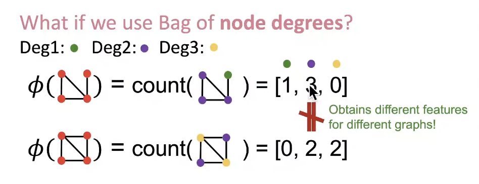
• Both Graphlet Kernel and Weisfeiler-Lehman (WL) Kernel use Bag-of-representation of graph, where is more sophisticated than node degrees!

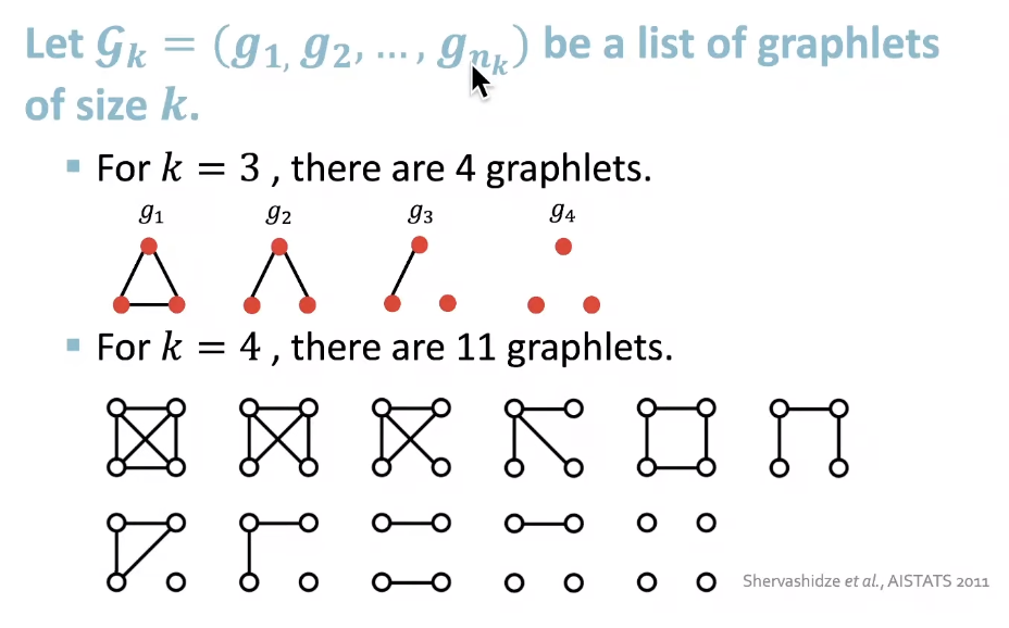
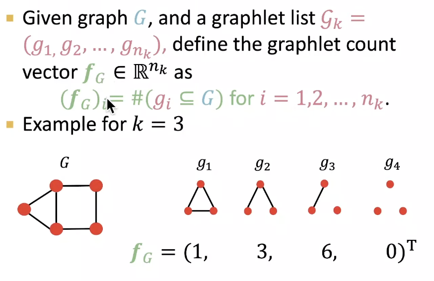
Graphlet Features

• Key Idea: Count the number of different graphlets in a graph
  ✓ Definition of graphlets here is slightly different from node-level features.
  ✓ The two differences are:
  • Nodes in graphlets here do not need to be connected
  • The graphlets here are not rooted.
  • Example:
    
    
• Given two graphs, G and G', graphlet kernel is computed as
  
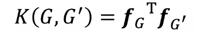
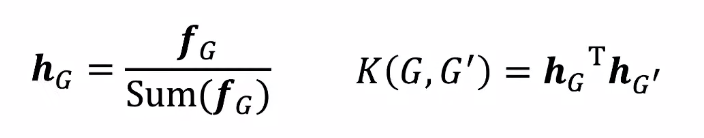
• Problem: if G and G' have different sizes, that will greatly skew the value.
• Solution: normalize each feature vector
  
• Limitations: Counting graphlets is expensive!
  ❍ Counting size-k graphlets for a graph with size n by enumeration takes n^k
  ❍ This is unavoidable in the worst-case since subgraph isomorphism test is NP-hard
  ❍ If a graph's node degree is bounded by d, an O(nd^{k-1}) algorithm exists to count all the graphlets of size k

Weisfeiler-Lehman Kernel

• Goal : design an efficient graph feature descriptor Φ(G)
• Idea: use neighborhood structure to iteratively enrich node vocabulary
  ❍ Generalized version of Bag of node degrees since node degrees are one-hop neighborhood information

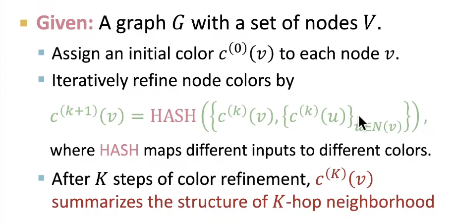
Color Refinement

• Example of color refinement given two graphs:
  
  →
  
  →
  
  →
  

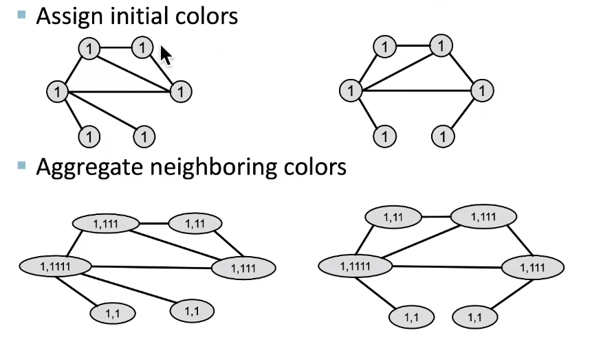
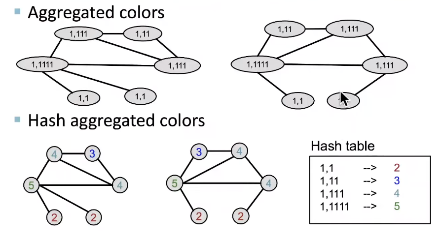
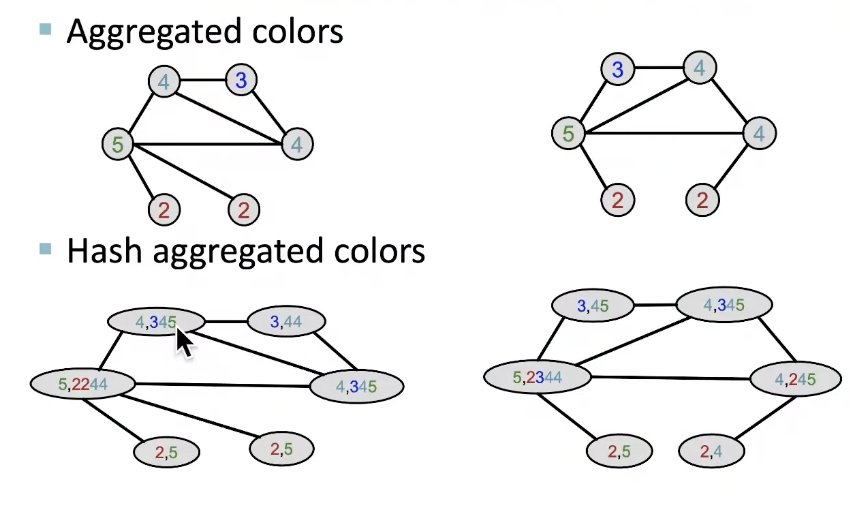
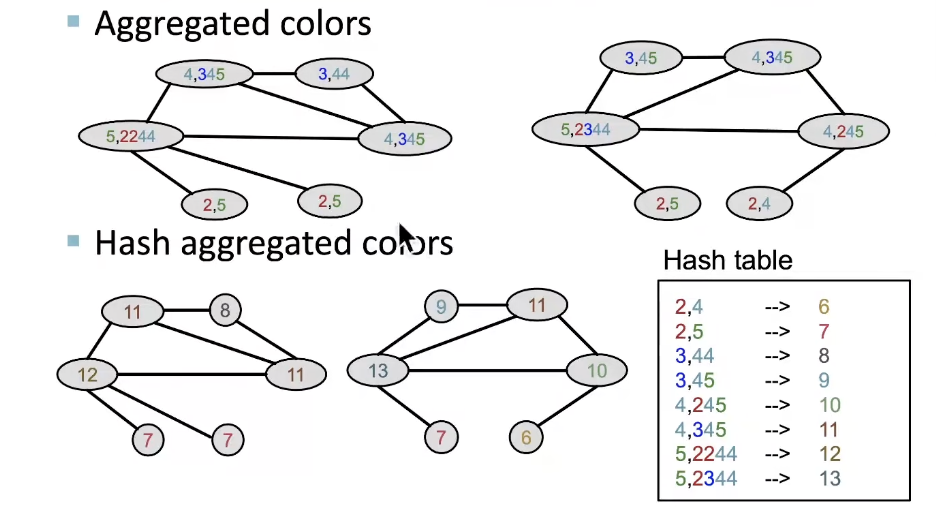
• After color refinement, WL kernel counts number of nodes with a given color.
  

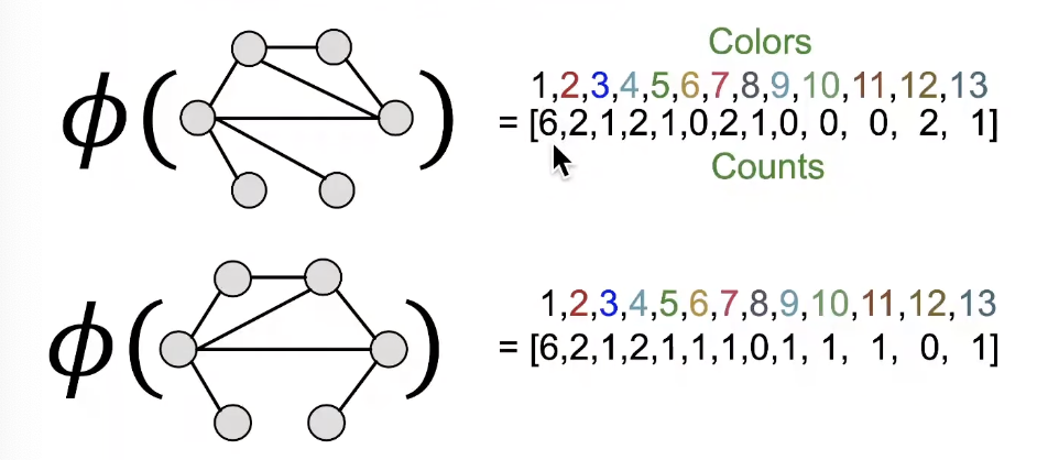
• The WL kernel value is computed by the inner product of the color count vectors:
  

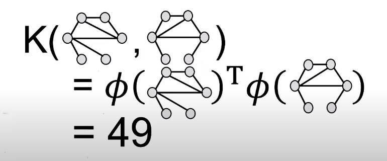
• WL kernel is computationally efficient
  ✓ The time complexity for color refinement at each step is linear in #(edges), since it involves aggregating neighboring colors.

• When computing a kernel value, only colors appeared in the two graphs need to be tracked.
  ✓ Thus, #(colors) is at most the total number of nodes.

• Counting colors takes linear-time w.r.t. #(nodes).

• In total, time complexity is linear in #(edges).