Recurrence resonance - noise-enhanced dynamics in recurrent neural networks

This paper introduces Recurrence Resonance (RR), where adding optimal white noise enhances the mutual information ($I$) between consecutive states, reflecting improved internal information flow. Using Symmetric Boltzmann Machines (SBMs) with varied weight matrices (random, Autapses-only, Hopfield, NRooks), the study shows that RR occurs in systems with multiple pre-existing attractors (fixed points, n-cycles) when trapped in one without noise. Optimal noise r_opt enables exploration of these attractors, increasing entropy ($H$) and $I$, while excessive noise disrupts predictability, reducing $I$.

What does it mean that adding noise

it means adding random signals (white noise, drawn from $N(0,1)$) to each neuron in the recurrent neural network (RNN). Specifically:

• Noise is introduced via $r \eta_n(t)$ in the input equation $u_n(t)$, where $r$ controls its strength too explore how noise affects the network’s dynamics and information processing. While noise is typically seen as disruptive, the paper shows it can enhance information flow under specific conditions, a phenomenon (RR)
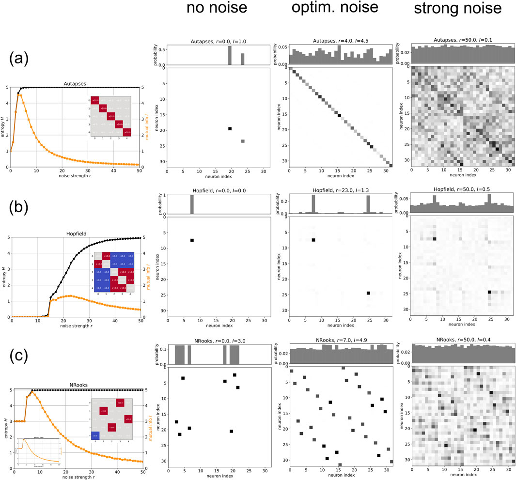
• Continuous noise was applied in most experiments, with strength $r$ varied to observe changes in entropy $H$, mutual information $I$, and divergence $D$ (Figures 1, 2).
  
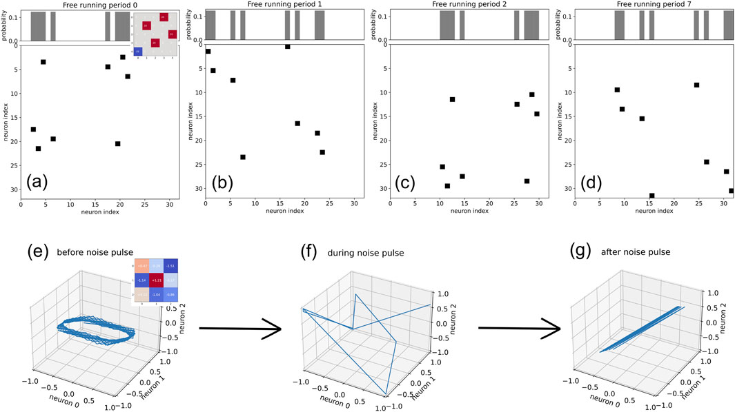
• Short noise pulses were also tested to switch attractors
  

Noise enables the exploration of already-existing multiple attractors

• Multiple attractors (e.g., fixed points, n-cycles) are predefined by the weight matrix $W$ and the network’s dynamics before noise is added (Section 3.1). Noise doesn’t create new attractors but allows the system to transition between them (Section 4).
• Without noise ($r = 0$), the system is trapped in one attractor; with optimal noise ($r_{opt}$), it visits more pre-existing attractors. Excessive noise ($r \gg r_{opt}$) randomizes transitions without forming new attractors

method to confirm that the system visits multiple attractors

They confirmed it using joint probability distributions and information-theoretic measures:

• Joint Probability $P(s(t), s(t+1))$: Calculated from state time series over $N_T$ steps, visualized as matrices (Figures 1D-F, 2 columns 2-4).
  • r = 0: Few states visited (trapped in one attractor).
  • r = r_opt: More states visited, clustered around attractors.
  • r = 50: Nearly all states visited randomly.
• Information Measures:
  • Entropy $H$: Measures state diversity (Equation 4).
  • Mutual Information $I$: Measures predictability between states, peaking at r_opt
  • Divergence $D = H - I$: Indicates randomness.
• State Transition Graphs: Showed preferred paths forming attractors as $w$ increases
• Specific Tests: Confirmed in Autapses-only (32 fixed points), Hopfield (2 fixed points), and NRooks (4 8-cycles) via $P(s(t), s(t+1))$ patterns

What kind of prior learning process allowed multiple attractors to already exist?

No explicit learning process was used; multiple attractors exist due to the weight matrix $W$ and inherent dynamics, not training.

• Mechanism:
  • $W$ is predefined (randomly or structurally), and the RNN’s feedback loops naturally form attractors like fixed points or cycles (Section 1, 2.1).
  • Example: Large $w$ creates stable attractors; small $w$ leads to randomness (Section 3.1.1).
• No Training: Unlike supervised learning, attractors emerge from the system’s autonomous dynamics (e.g., NRooks’ permutation-like $W$ ensures cycles, Section 3.2.3).
• Exception: Hopfield’s $W$ was designed to store two patterns, implying a minimal "learning" setup, but this was pre-set, not trained in the study (Section 3.2.2).
• Conclusion: Attractors are a mathematical consequence of $W$ and dynamics, assumed to exist for studying noise effects (Section 4).

Weight matrix design (Random, Autapses-only, Hopfield, NRooks)

Random Gaussian Matrix

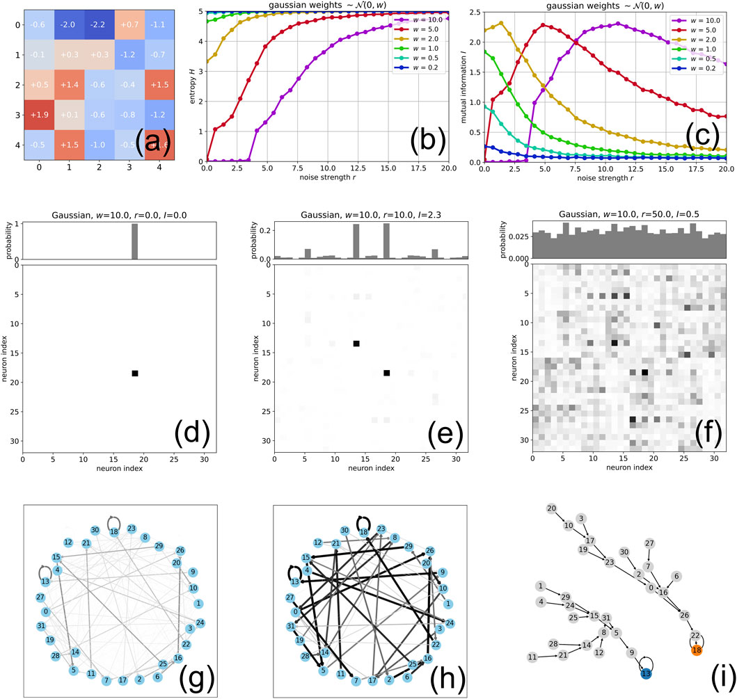
• Design: $w_{nm} \sim N(0, 1)$, scaled by $w$ (Section 3.1, Figure 1A).
• Attractors:
  • Small $w$: No clear attractors (random walk).
  • Large $w$: Fixed points or cycles (e.g., Figure 1I shows 2 fixed points at $w = 5$).
• Effect: Noise shifts from one attractor ($r = 0$) to multiple ($r_{opt}$), then randomness ($r = 50$).

Autapses-only

• Design: Diagonal $w = +10$, others 0 (Section 3.2.1, Figure 2A).
• Attractors: 32 quasi-stable fixed points (5 neurons, $2^5$), each neuron persists independently.
• Plot (Figure 2A):
  • $r = 0$: $H \approx 1$, $I \approx 1$ (2 points).
  • $r = 4$ (optimal): $H \approx 5$, $I \approx 4.5$ (all points visited).
  • $r = 50$: $H \approx 5$, $I \approx 0.1$ (random transitions).

Hopfield

• Design: Symmetric, stores two patterns (24, 7), no self-connections (Section 3.2.2, Figure 2B).
• Attractors: 2 stable fixed points corresponding to stored patterns.
• Plot (Figure 2B):
  • $r = 0$: $H = 0$, $I = 0$ (trapped in 24).
  • $r = 23$ (optimal): $H \approx 1.5$, $I \approx 1.3$ (both visited).
  • $r = 50$: $H$ increases, $I$ drops slightly.

NRooks

• Design: One non-zero ($w = 20$) per row/column (Section 3.2.3, Figure 2C).
• Attractors: 4 stable 8-cycles (32 states organized into cycles).
• Plot (Figure 2C):
  • $r = 0$: $H = 3$, $I = 3$ (one cycle).
  • $r = 7$ (optimal): $H \approx 5$, $I \approx 4.9$ (all cycles).
  • $r = 50$: $H \approx 5$, $I$ decreases (randomness).