Paper Review

요약

Residual Learning(잔차 학습)은 레이어의 입력을 Reference로 하는 Deep Learning 기법이다.

ResNet은 기존 모델에 비해 상당한 깊이에서도 높은 정확도를 유지할 뿐 아니라, 빠른 학습 시간을 보여준다. ILSVRC 2015에서 우승하였으며 CIFAR 10, 100 1000 image classification과 Detection, Localization, Segmentation에서도 뛰어난 성능을 보인다.

Introduction

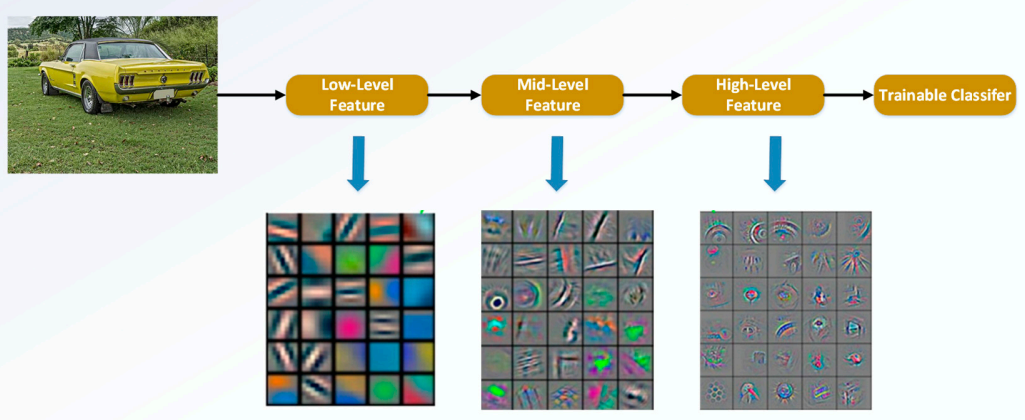
Deep Network는 입력에 가까울수록 지역적인 low feature가, 출력에 가까울수록 전역적이고 추상적인 high feature가 나타난다. 깊이에 따라 이러한 feature level이 다양해지므로 network 깊이는 중요한 요소라고 할 수 있다.

그렇다면 layer가 많으면 많을 수록 좋은 network일까?

기존에 존재하던 기울기 소실/폭발 문제는 초기 정규화(normalized initialization)와 중간 정규화 층(intermediate normalization layer)을 통해 어느정도 해결됐다.

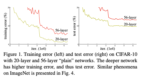
하지만 network가 점점 깊어지면서 degradation이라는 새로운 문제가 발생한다. degradation은 deeper network의 정확도가 포화(saturated)되었다가 급격히 저하(degraded)되는 것을 뜻한다.

degradation은 높은 traning error를 보인다는 점에서, 높은 training accuracy를 보이는 과적합(overfitting)과는 별개의 문제라고 할 수 있다.

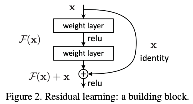
저자는 이러한 문제를 해결하기 위해 Deep Residual Learning 구조를 제안한다. 입력이 x, relu를 거치기 이전의 출력이 H(x)라면, H(x) = F(x) + x 로 나타낼 수 있다. 이와 같이 입력이 층을 건너뛰는 것을 skip connection 이라고 한다.

본 논문에서는 skip connection을 identity mapping 즉, 다른 추가적인 파라미터나 연산없이 구현하였다. 이로써 전체 network는 여전히 확률적 경사하강법(Stochastic Gradient Descent)을 통해 E2E 학습을 진행할 수 있다.

Deep Residual Learning

Residual Learning (잔차 학습)

그렇다면 H(x) = F(x) + x 와 같은 새로운 구조를 제시한 이유는 무엇일까? x는 우리가 이미 알고 있는 값이므로 관점을 바꾸어 F(x) = H(x) - x 를 학습시킨다고 생각해보자.

만약 정답의 형태가 H(x) = x 와 같은 identity mapping이라면 Residual Learning에서는 F(x) = 0 이 되야 하므로 이러한 결과가 나오도록 학습시키는 것이 (Residual Learning이 아닌) plain network가 H(x) = x가 되도록 학습시키는 것보다 훨씬 쉽기 때문이다.

물론 항상 정답이 H(x) = x 가 되는 것은 아니지만 아무것도 없는 상태에서 multiple layers를 어떤 함수에 근사 시키는 것보다는 x라는 reference를 제공하는 identity mapping을 바탕으로 정답을 찾아나가는 것이 학습에 유리하다.

Identity Mapping by Shortcuts

identity mapping은 아래와 같이 나타낼 수 있다

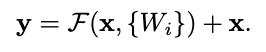
Figure 2를 예시로 들면 F = W2σ(W1x)인데, σ는 ReLU 함수이고 bias는 표기상의 편의를 위해 빠졌다. F + x 연산은 shortcut connection과 element-wise addition으로 수행된다.

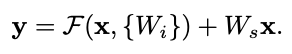
행렬 덧셈의 특성상 F와 x의 차원이 같아야 하는데, 만약 그렇지 않을 경우에는 차원을 맞추기 위해 Ws를 x에 곱한 후 더해준다.

Network Architectures(for ImageNet)

Plain Network

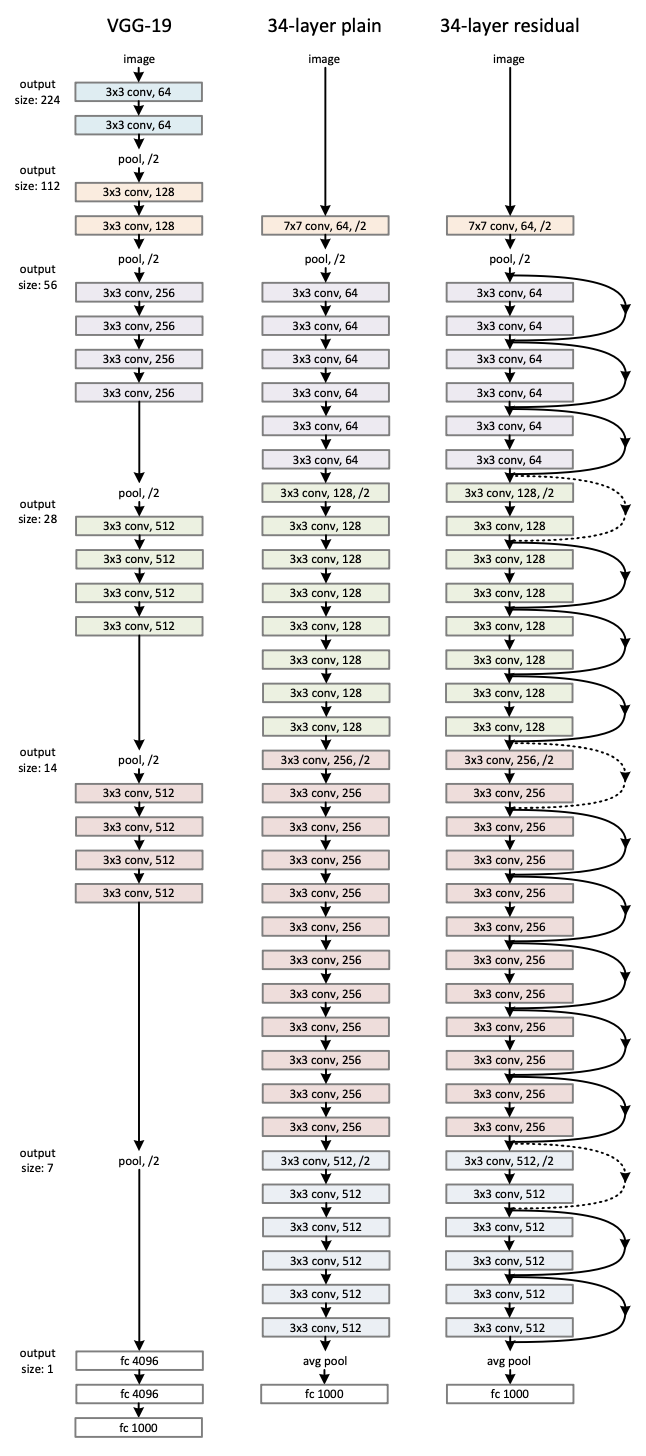
VGG Net(Fig.3 왼쪽)에서와 같이 convolutional layer는 거의 3x3 필터를 사용하고 두가지 디자인 규칙을 적용한다.

1. 동일한 feature map size에 대해서 각 layer는 똑같은 수의 filter를 가진다.
2. 만약 feature map size가 절반이 되면, filter의 수는 두배로 늘린다.

이는 매 layer의 시간 복잡성을 유지하기 위함이다.

여기에 convolutional layer(stride=2)로 직접 downsampling을 수행한다. 마지막에는 global average pooling과 함께 1000-way fully-connected Layer 및 softmax를 통해 분류를 진행하게 된다.(Fig.3 가운데)

Residual Network

Plain Network에서 identity mapping이 추가된다. 차원이 증가할 때는 점선으로 표기하였는데 두 가지 선택지를 고려할 수 있다.

(A) identity mapping을 수행하고 증가한 차원 부분에 대해서는 zero padding을 적용한다.
(B) projection shortcut을 사용한다(Ws, 1x1 conv).

두 경우 모두 size가 반으로 줄어드므로 stride를 2로 설정하였다.

Implemetation

실제 구현은 아래와 같이 진행한다.

1. 이미지의 짧은 쪽이 256~480 사이가 되도록 리사이즈를 진행한다.
2. 224x224 사이즈만큼 추출한다(기존 or 좌우 반전) + per-pixel 평균을 뺸다.
3. standard color augmentation 적용
4. Batch Normalization을 convolution ~ activation 사이에 적용한다.
5. He 초기화 방법으로 가중치 초기화
6. SGD 적용 (mini-batch size : 256)
7. Learning rate 0.1에서 시작하여 10씩 나눠주며 진행
8. iteration: 60e4, Weight decay: 0.0001, Momentum: 0.9, dropout X

테스트 시에는 10-crop testing을 적용하였고, muliple scale을 사용해 짧은 쪽의 길이가 {224, 256, 384, 480, 640} 중 하나가 되게 한다.

Experiments

ImageNet Classification

ImageNet 2012 데이터셋이 사용되었는데 128만개의 training images, 5만개의 validation images, 10만개의 test images가 사용 되었고, top-1 & top-5 error rates를 측정하였다.

Plain Networks

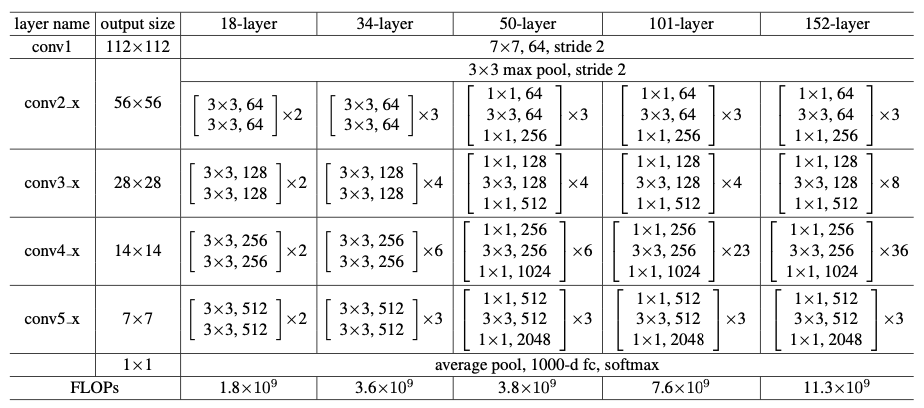
처음에는 18-layer와 34-layer에 대한 평가를 진행하였다. 18-layer는 아까 위에서 보았던 34-layer와 유사한 형태이다. 아래 그래프를 통해 알 수 있듯이 더 깊은 34-layer가 18-layer보다 높은 validation error(굵은 선)를 보인다.

또한 초반부에 설명했던 degradation 문제 또한 발생하였다. 즉, 34-layer plain network의 training error(가는 선)가 전체 학습 과정에서 가장 높게 나타났다.

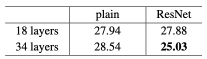
plain network에서는 34-layer에서 validation error가 커지며 degradation 문제가 발생하였다.

이러한 문제는 배치 정규화가 적용되어 순전파/역전파 기울기에는 문제가 없었기 때문에 기울기 소실에 의해 일어나는 것으로 판단되지는 않는다.

Residual Networks

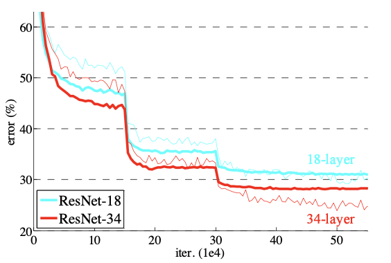
다음으로는 plain network에 residual learning이 적용된 ResNet-18과 ResNet-34의 성능을 측정하였다. 이때 모든 shortcut에 대해서 차원이 증가될 때 zero padding(A 옵션)을 적용하였다. zero padding은 추가적인 파라미터가 필요하지 않으므로 plain 모델과 파라미터 수의 차이는 없다.

위 결과들을 토대로 몇가지 사실을 알 수 있다.

1. ResNet-34는 ResNet-18 보다 뛰어난 성능을 보이며(약 2.8%) 낮은 traning error가 눈에 띈다. => 이를 통해 degradation 문제가 해소되었음을 알 수 있다.
2. plain network와 비교하였을 때, 34-layer ResNet은 top-1 error rate를 약 3.5% 개선시켰다.(28.54% -> 25.03%)
3. 18-layer plain/residual net 모두 상당한 정확도를 보였지만, 18-layer ResNet이 조금 더 빨리 수렴하였다.

network가 엄청나게 깊지 않다면(18-layer 포함), SGD solver는 여전히 plain net에 훌륭한 solution을 찾아줄 수 있다.

물론 ResNet은 여기에 빠른 수렴을 통해 최적화를 쉽게 만들어준다.

Identity vs. Projection Shortcuts

앞에서 파라미터가 필요하지 않은 identity shortcut이 학습에 도움이 되는 것을 알 수 있었는데, 이번에는 zero padding과 projection shortcut을 비교하여 살펴본다.

세 가지 옵션이 있다.

A) increasing dimension에 zero padding shortcut이 사용된 경우. 모든 shortcut은 parameter-free이다.

B) increasing dimension에 projection shortcut을 적용하고 나머지는 identity shortcut인 경우.

C) projection shorcut만 사용한 경우

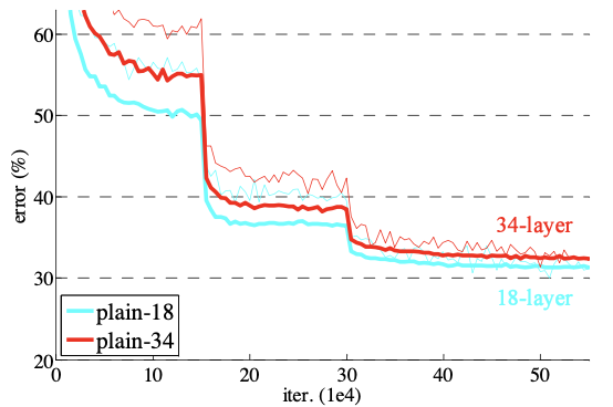
Error rates (%, 10-crop testing) on ImageNet validation. VGG-16 is based on our test. ResNet-50/101/152 are of option B that only uses projections for increasing dimensions.

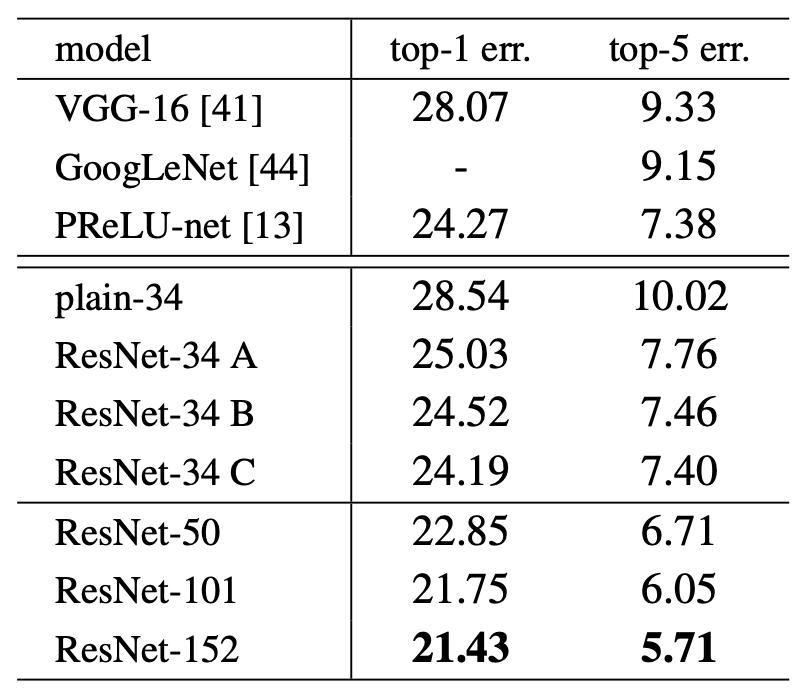
위 Table에서 알 수 있는 것은 우선 모두 plain보다는 상당히 좋은 성능을 보였다는 것이다.

ABC 끼리 차이는 있지만(A<B<C) degradation 문제를 해결하는데에 필수적이지는 않으므로 편의를 위해 C는 사용하지 않았다.

bottleneck architecture의 복잡성을 높이지 않는 데에 Identical shortcuts가 중요함.

Deeper Bottleneck Architectures

ResNet의 깊이가 깊어짐에 따라 training time이 너무 커지는 것을 막기 위해 파라미터 수가 적은 bottleneck architecture를 도입하였다.

위 아래에 있는 1x1 conv layer는 각각 차원을 줄였다가 다시 늘리는 데에 사용된다.

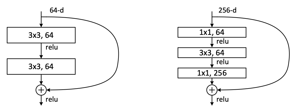
이렇게 다시 차원을 원래대로 돌아오도록 하는 이유는 parameter-free인 identity shortcut이 bottleneck architecture에 매우 중요하기 때문이다.

만약 identity shortcut이 projection으로 교체된다면 2개의 high-dimentional 출력이 연결되어 시간 복잡도와 모델 크기가 두배가 된다.

이러한 결과를 막아주기 때문에 identity shortcut은 bottleneck design이 효과적인 모델이 되는데 중요한 역할을 한다.

50-layer ResNet

50-layer부터는 기존의 2-layer block을 3-layer bottleneck block으로 교체한다. 이 때 B 옵션을 사용하였다.

101-layer and 152-layer ResNets

Error rates (%) of single-model results on the ImageNet validation set (except † reported on the test set).

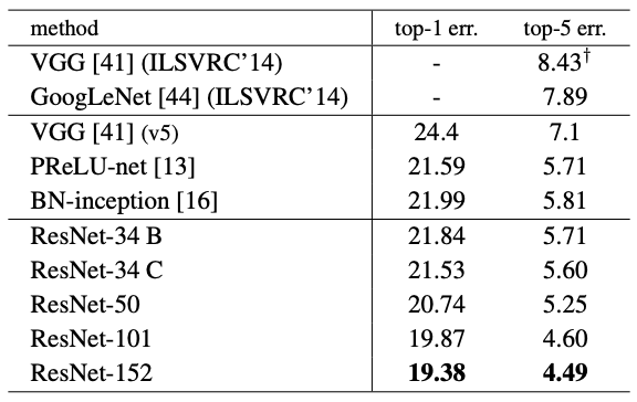
더 많은 3-layer block들을 사용하여 101-layer, 152-layer ResNet을 구성하였는데, 놀랍게도 깊이가 상당히 늘어났음에도 불구하고 152-layer ResNet(11.3 billion FLOPs)은 여전히 VGG-16/19 nets(15.3/19.6 billion FLOPs)보다 더 낮은 복잡도를 가졌다.

위 single-model 테스트에서 34-layer ResNets이 매우 경쟁력 있는 정확도를 보이지만, 50/101/152-layer ResNet은 더 높은 정확도를 보인다. 또한 여전히 degradation 문제를 찾아볼 수 없었다.

152-layer ResNet은 single-model 테스트에서 4.49%의 top-5 validation error를 보여주었는데, 이것은 심지어 single-model 임에도 이전의 모든 앙상블 모델을 제친 것이다.

Comparisons with State-of-the-art Methods

Error rates (%) of ensembles. The top-5 error is on the test set of ImageNet and reported by the test server.

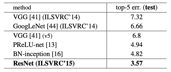
저자는 서로 다른 깊이의 6개 모델을 앙상블한 모델을 만들었고, 이는 3.57% top-5 error를 보여주었다. 이 모델은 ILSVRC 2015에서 우승을 차지하였다.

Pytorch Implementation (18-layer)

ResNet은 위 표처럼 Block이 반복되는 구조이므로 Block 코드를 먼저 작성한 후, 이를 바탕으로 ResNet을 구성한다.

Block을 쌓는 구조이기 때문에 ResNet-18을 만들 수 있다면 34, 50 등도 만들 수 있다.

Import

import torch
from torch import nn
from torch import Tensor
from typing import Optional, Callable, Union, Type, List

구조만 파악하기 때문에 학습 관련 라이브러리는 배제하였다.

convolutional layer

def conv3x3(in_planes: int, out_planes: int, stride: int = 1, groups: int = 1, dilation: int = 1) -> nn.Conv2d:
    """3x3 convolution with padding"""
    return nn.Conv2d(in_planes, out_planes, kernel_size=3, stride=stride, padding=dilation, groups=groups, bias=False, dilation=dilation)

def conv1x1(in_planes: int, out_planes: int, stride: int = 1) -> nn.Conv2d:
    """1x1 convolution"""
    return nn.Conv2d(in_planes, out_planes, kernel_size=1, stride=stride, bias=False)

BasicBlock과 Bottleneck에서 사용될 3x3, 1x1 convolutional layer를 정의하는 부분.

BasicBlock

class BasicBlock(nn.Module):
    def __init__(
        self,
        inplanes: int,
        planes: int,
        stride: int = 1,
        downsample: Optional[nn.Module] = None,
        groups: int = 1,
        dilation: int = 1,
        norm_layer: Optional[Callable[..., nn.Module]] = None
    )-> None:
        super(BasicBlock, self).__init__()

        # Normalization Layer
        if norm_layer is None:
            norm_layer = nn.BatchNorm2d
        
        self.conv1 = conv3x3(inplanes, planes, stride) # padding, dilation = 1
        self.bn1 = norm_layer(planes)
        self.relu = nn.ReLU(inplace=True) # inplace : 원본 직접 수정 여부
        self.conv2 = conv3x3(planes, planes) # stride = 1
        self.bn2 = norm_layer(planes)
        self.downsample = downsample
        self.stride = stride

    def forward(self, x: Tensor) -> Tensor:
        identity = x

        out = self.conv1(x)
        out = self.bn1(out)
        out = self.relu(out)

        out = self.conv2(out)
        out = self.bn2(out)

        if self.downsample is not None:
            identity = self.downsample(x)
        
        out += identity  #  residual connection
        out = self.relu(out)
        return out

정규화는 기본값으로 2d Batch Normalization이 사용된다.

Block 구성)
conv3x3 - BN - ReLU - conv3x3 - BN - residual connection - ReLU

Bottleneck

class Bottleneck(nn.Module):
    # Bottleneck in torchvision places the stride for downsampling at 3x3 convolution(self.conv2)
    # while original implementation places the stride at the first 1x1 convolution(self.conv1)
    # according to "Deep residual learning for image recognition"https://arxiv.org/abs/1512.03385.
    # This variant is also known as ResNet V1.5 and improves accuracy according to
    # https://ngc.nvidia.com/catalog/model-scripts/nvidia:resnet_50_v1_5_for_pytorch.

    expansion: int = 4

    def __init__(
        self,
        inplanes: int,
        planes: int,
        stride: int = 1,
        downsample: Optional[nn.Module] = None,
        groups: int = 1,
        base_width: int = 64,
        dilation: int = 1,
        norm_layer: Optional[Callable[..., nn.Module]] = None,
    ) -> None:
        super().__init__()
        if norm_layer is None:
            norm_layer = nn.BatchNorm2d
        width = int(planes * (base_width / 64.0)) * groups
        # Both self.conv2 and self.downsample layers downsample the input when stride != 1
        self.conv1 = conv1x1(inplanes, width)
        self.bn1 = norm_layer(width)
        self.conv2 = conv3x3(width, width, stride, groups, dilation)
        self.bn2 = norm_layer(width)
        self.conv3 = conv1x1(width, planes * self.expansion)
        self.bn3 = norm_layer(planes * self.expansion)
        self.relu = nn.ReLU(inplace=True)
        self.downsample = downsample
        self.stride = stride

    def forward(self, x: Tensor) -> Tensor:
        identity = x

        out = self.conv1(x)
        out = self.bn1(out)
        out = self.relu(out)

        out = self.conv2(out)
        out = self.bn2(out)
        out = self.relu(out)

        out = self.conv3(out)
        out = self.bn3(out)

        if self.downsample is not None:
            identity = self.downsample(x)

        out += identity
        out = self.relu(out)

        return out

Bottleneck은 ResNet-18에서 사용되지 않는다. 자세한 내용은 레퍼런스에서 참고할 수 있다.

ResNet-18

class ResNet(nn.Module):
    def __init__(
        self,
        block: Type[Union[BasicBlock, Bottleneck]],
        layers: List[int],
        num_classes: int = 1000,
        zero_init_residual: bool = False,
        norm_layer: Optional[Callable[..., nn.Module]] = None
    )-> None:
        super(ResNet, self).__init__()
        if norm_layer is None:
            norm_layer = nn.BatchNorm2d
        self._norm_layer = norm_layer # batch norm layer
        
        self.inplanes = 64 # input shape
        self.dilation = 1 # dilation fixed
        self.groups = 1 # groups fixed
        
		# input block
        self.conv1 = nn.Conv2d(3, self.inplanes, kernel_size=7, stride=2, padding=3, bias=False)
        self.bn1 = norm_layer(self.inplanes)
        self.relu = nn.ReLU(inplace=True)
        self.maxpool = nn.MaxPool2d(kernel_size=3, stride=2, padding=1)
        
		# residual blocks
        self.layer1 = self._make_layer(block, 64, layers[0])
        self.layer2 = self._make_layer(block, 128, layers[1], stride=2, dilate=False)
        self.layer3 = self._make_layer(block, 256, layers[2], stride=2, dilate=False)
        self.layer4 = self._make_layer(block, 512, layers[3], stride=2, dilate=False)
        self.avgpool = nn.AdaptiveAvgPool2d((1, 1))
        self.fc = nn.Linear(512, num_classes)
        
		# weight initialization
        for m in self.modules():
            if isinstance(m, nn.Conv2d):
                nn.init.kaiming_normal_(m.weight, mode='fan_out', nonlinearity='relu')
            elif isinstance(m, (nn.BatchNorm2d, nn.GroupNorm)):
                nn.init.constant_(m.weight, 1)
                nn.init.constant_(m.bias, 0)

        # Zero-initialize the last BN in each residual branch,
        # so that the residual branch starts with zeros, and each residual block behaves like an identity.
        # This improves the model by 0.2~0.3% according to https://arxiv.org/abs/1706.02677
        if zero_init_residual:
            for m in self.modules():
                if isinstance(m, Bottleneck):
                    nn.init.constant_(m.bn3.weight, 0)  # type: ignore[arg-type]
                elif isinstance(m, BasicBlock):
                    nn.init.constant_(m.bn2.weight, 0)  # type: ignore[arg-type]
                    
    def _make_layer(self, block: Type[Union[BasicBlock, Bottleneck]], planes: int, blocks: int, stride: int=1, dilate: bool = False) -> nn.Sequential:
        norm_layer = self._norm_layer
        downsample = None
        
		# downsampling 필요할 경우 downsample layer 생성
        if stride != 1 or self.inplanes != planes:
            downsample = nn.Sequential(
                conv1x1(self.inplanes, planes, stride),
                norm_layer(planes)
			)
            
        layers = []
        layers.append(block(self.inplanes, planes, stride, downsample, self.groups, self.dilation, norm_layer))
        self.inplanes = planes
        for _ in range(1, blocks):
            layers.append(block(self.inplanes, planes, groups=self.groups, dilation=self.dilation, norm_layer=norm_layer))

        return nn.Sequential(*layers)
    
    def forward(self, x: Tensor) -> Tensor:
        print('input shape:', x.shape)
        x = self.conv1(x)
        print('conv1 shape:', x.shape)
        x = self.bn1(x)
        print('bn1 shape:', x.shape)
        x = self.relu(x)
        print('relu shape:', x.shape)
        x = self.maxpool(x)
        print('maxpool shape:', x.shape)

        x = self.layer1(x)
        print('layer1 shape:', x.shape)
        x = self.layer2(x)
        print('layer2 shape:', x.shape)
        x = self.layer3(x)
        print('layer3 shape:', x.shape)
        x = self.layer4(x)
        print('layer4 shape:', x.shape)

        x = self.avgpool(x)
        print('avgpool shape:', x.shape)
        x = torch.flatten(x, 1)
        print('flatten shape:', x.shape)
        x = self.fc(x)
        print('fc shape:', x.shape)

        return x

ResNet 코드에서는 BasicBlock을 이용하여 Residual Blocks를 구성하는 _make_layer 함수를 구현하고 이를 통해서 Block을 쌓는다.

또한 입력 맨 처음 단의 Input Block 또한 별도로 구성되어 있다.

Result

model = ResNet(BasicBlock, [2, 2, 2, 2])
x = torch.randn(1, 3, 112, 112)
print('\noutput shpae: ', model(x).shape)

ResNet-18은 각 블럭이 2개씩 구성되어 있으므로 [2, 2, 2, 2]를 입력한다.

input shape: torch.Size([1, 3, 112, 112])
conv1 shape: torch.Size([1, 64, 56, 56])
bn1 shape: torch.Size([1, 64, 56, 56])
relu shape: torch.Size([1, 64, 56, 56])
maxpool shape: torch.Size([1, 64, 28, 28])
layer1 shape: torch.Size([1, 64, 28, 28])
layer2 shape: torch.Size([1, 128, 14, 14])
layer3 shape: torch.Size([1, 256, 7, 7])
layer4 shape: torch.Size([1, 512, 4, 4])
avgpool shape: torch.Size([1, 512, 1, 1])
flatten shape: torch.Size([1, 512])
fc shape: torch.Size([1, 1000])

output shpae: torch.Size([1, 1000])

레퍼런스

Deep Residual Learning for Image Recognition(2015) - 논문
ResNet 논문 리뷰 - Youtube
Short Connection과 Identity Mapping - 블로그
ResNet 논문 리뷰 - 블로그
Pytorch 구현 - 블로그