[데이터분석] 자전거 수요 예측

Jaewon Lim·2024년 11월 28일

🌐 개요

자전거 대여 시스템 데이터 분석

자전거 대여 패턴을 분석하여 자전거 배치 및 운영 전략을 최적화하고, 대여 수요를 예측하는 것. 이를 통해 대여 시스템의 효율성을 높이고 사용자 만족도를 증가시키는 방법을 찾는다.
최종 목표는 RMSLE를 최대한 낮추는 것.

RMSLE(Root Mean Squared Logarithmic Error)란?
예측 값과 실제 값의 차이를 로그 변환하여 계산한 후, 그 차이의 제곱 평균의 제곱근을 구한 값. 예측 오차를 측정하는 데 사용되며, 큰 값보다 작은 값의 오차를 더 중요시 하는 경우에 사용된다. 이는 예측 값이 실제 값보다 훨씬 클 때 더 큰 패널티를 부과하므로, 예측 값이 과대평가 되는 것을 방지한다.

📊 사용 데이터 셋

train.csv : count 컬럼이 포함되어 있으며, 예측 대상인 종속 변수
test.csv : casual, registered, count 컬럼이 포함되어 있지 않음
casual과 registered 는 자전거 대여 수요를 예측하는데 참고하며, count는 두 컬럼간의 합

컬럼명	데이터 타입	설명
datetime	datetime	자전거 대여 기록의 날짜 및 시간. 예시: 2011-01-01 00:00:00
season	int	계절 (1: 봄, 2: 여름, 3: 가을, 4: 겨울)
holiday	int	공휴일 여부 (0: 평일, 1: 공휴일)
workingday	int	근무일 여부 (0: 주말/공휴일, 1: 근무일)
weather	int	날씨 상황 (1: 맑음, 2: 구름낌/안개, 3: 약간의 비/눈, 4: 폭우/폭설)
temp	float	실측 온도 (섭씨)
atemp	float	체감 온도 (섭씨)
humidity	int	습도 (%)
windspeed	float	풍속 (m/s)
casual	int	등록되지 않은 사용자의 대여 수
registered	int	등록된 사용자의 대여 수
count	int	총 대여 수 (종속 변수)

🔍 데이터 셋 EDA

데이터 분포 시각화 - 1

범주형 데이터 변환

season, holiday, workingday, weather 컬럼이 범주형 데이터 이어야한다.

category_list = ['season', 'holiday', 'workingday', 'weather']
for var in category_list:
    train_df[var] = train_df[var].astype('category')
    test_df[var] = test_df[var].astype('category')
    
# Mapping numbers to understandable text
season_dict = {1:'Spring', 2:'Summer', 3:'Fall', 4:'Winter'}
weather_dict = {1:'Clear', 2:'Misty+Cloudy', 3:'Light Snow/Rain', 4:'Heavy Snow/Rain'}
train_df['season'] = train_df['season'].map(season_dict)
train_df['weather'] = train_df['weather'].map(weather_dict)

test_df['season'] = test_df['season'].map(season_dict)
test_df['weather'] = test_df['weather'].map(weather_dict)

train_df.head(n=3)

컬럼별 분포 (날씨, 계절, 근무날)

# Average values across each of the categorical columns 
fig = plt.figure(figsize=(15,10))

axes = fig.add_subplot(2, 2, 1)
group_weather = pd.DataFrame(train_df.groupby(['weather'])['count'].mean()).reset_index()
sns.barplot(data=group_weather, x='weather', y='count', ax=axes)
axes.set(xlabel='Weather', ylabel='Count', title='Average bike rentals across Weather')

axes = fig.add_subplot(2, 2, 2)
group_season = pd.DataFrame(train_df.groupby(['season'])['count'].mean()).reset_index()
sns.barplot(data=group_season, x='season', y='count', ax=axes)
axes.set(xlabel='Season', ylabel='Count', title='Average bike rentals across Seasons')

axes = fig.add_subplot(2, 2, 3)
group_workingday = pd.DataFrame(train_df.groupby(['workingday'])['count'].mean()).reset_index()
sns.barplot(data=group_workingday, x='workingday', y='count', ax=axes)
axes.set(xlabel='Working Day', ylabel='Count', title='Average bike rentals across Working Day')

axes = fig.add_subplot(2, 2, 4)
group_season = pd.DataFrame(train_df.groupby(['holiday'])['count'].mean()).reset_index()
sns.barplot(data=group_season, x='holiday', y='count', ax=axes)
axes.set(xlabel='Holiday', ylabel='Count', title='Average bike rentals across Holiday')
plt.show()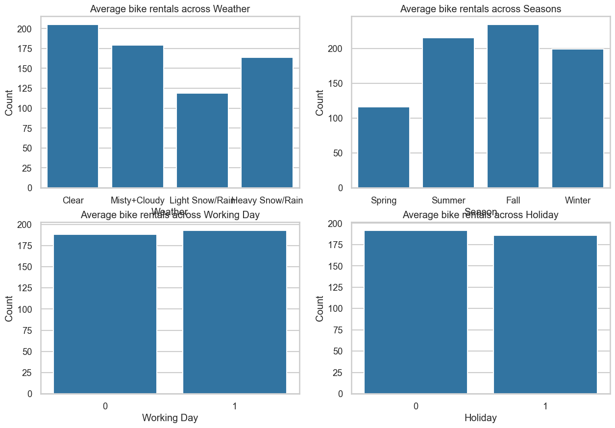

# Seaborn boxplots to get an idea of the distribution/outliers
f, axes = plt.subplots(2, 2, figsize=(15, 12))
hue_order= ['Clear', 'Heavy Snow/Rain', 'Light Snow/Rain', 'Misty+Cloudy']
sns.boxplot(data=train_df, y='count', x='weather', ax=axes[0][0], order=hue_order)
sns.boxplot(data=train_df, y='count', x='workingday', ax=axes[0][1])
hue_order= ['Fall', 'Spring', 'Summer', 'Winter']
sns.boxplot(data=train_df, y='count', x='season', ax=axes[1][0], order=hue_order)
sns.boxplot(data=train_df, y='count', x='holiday', ax=axes[1][1])

plt.show()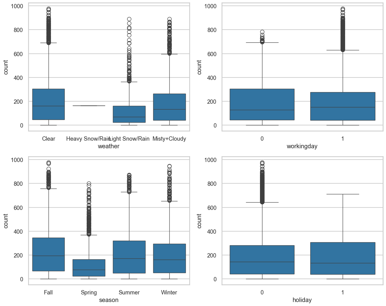

온도별 분포

평일과 휴일로 데이터를 나누어 온도별로 카운트 분포를 확인한다.

# Splitting data into working-day and non-working day
mydata_w = train_df[train_df.workingday==1]
mydata_nw = train_df[train_df.workingday==0]

bin_size = 4
mydata_w['temp_round'] = mydata_w['temp']//bin_size
mydata_nw['temp_round'] = mydata_nw['temp']//bin_size

mean_count_vs_temp_w = mydata_w.groupby('temp_round')['count'].mean()
mean_count_vs_temp_nw = mydata_nw.groupby('temp_round')['count'].mean()
idx_w, idx_nw = range(len(mean_count_vs_temp_w)), range(len(mean_count_vs_temp_nw))
labels_w = [str(bin_size*i)+' to '+str(bin_size*(i+1)) for i in range(len(mean_count_vs_temp_w))]
labels_nw = [str(bin_size*i)+' to '+str(bin_size*(i+1)) for i in range(len(mean_count_vs_temp_nw))]

fig = plt.figure(figsize=(18, 6))
axes = fig.add_subplot(1, 2, 1)
plt.bar(x=idx_w, height=mean_count_vs_temp_w)
plt.xticks(idx_w, labels_w, rotation=90)
plt.xlabel('temp bins')
plt.ylabel('Average Count')
plt.title('Working Days: Average Count given across temperature range')

axes = fig.add_subplot(1, 2, 2)
plt.bar(x=idx_nw, height=mean_count_vs_temp_nw)
plt.xticks(idx_nw, labels_nw, rotation=90)
plt.xlabel('temp bins')
plt.ylabel('Average Count')
plt.title('Non-Working Days: Average Count given across temperature range')

plt.show()

핏처 엔지니어링 - 1

Datetime 을 월별,일별,일수,시간 별 추가 카테고리를 만든다.

# Convert the 'datetime' column to a proper datetime format
train_df['datetime'] = pd.to_datetime(train_df['datetime'])
test_df['datetime'] = pd.to_datetime(test_df['datetime'])

# Extract components from the 'datetime' column
train_df['month'] = train_df['datetime'].dt.month
train_df['date'] = train_df['datetime'].dt.day
train_df['hour'] = train_df['datetime'].dt.hour
train_df['day'] = train_df['datetime'].dt.weekday

test_df['month'] = test_df['datetime'].dt.month
test_df['date'] = test_df['datetime'].dt.day
test_df['hour'] = test_df['datetime'].dt.hour
test_df['day'] = test_df['datetime'].dt.weekday

# Convert these columns to categorical types
category_list = ['month', 'date', 'hour', 'day']
for var in category_list:
    train_df[var] = train_df[var].astype('category')
    test_df[var] = test_df[var].astype('category')

# Mapping 0 to 6 day indices to Monday to Saturday 
day_dict = {0:'Monday', 1:'Teusday', 2:'Wednesday', 3:'Thursday', 4:'Friday', 5:'Saturday', 6:'Sunday'}
train_df['day'] = train_df['day'].map(day_dict)
test_df['day'] = test_df['day'].map(day_dict)

train_df.head(n=3)

데이터 분포 시각화 - 2

시간별 분포

시간별 데이터를 분리했으나, 하루 중 시간별로 분포를 표시한다.

# seaborn boxplots across hours
f, axes = plt.subplots(1, 1, figsize=(15, 6))
sns.boxplot(data=train_df, y='count', x='hour', hue='workingday', ax=axes)
handles, _ = axes.get_legend_handles_labels()
axes.legend(handles, ['Not a Working Day', 'Working Day'])
axes.set(title='Hourly Count based on Working day or not')

plt.show()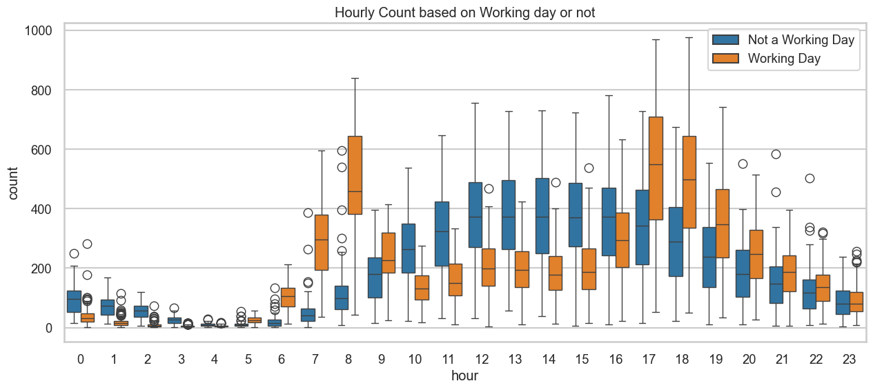

다양한 범주에 따라 시간별 평균 자전거 대수를 표시한다.


# Plots of average count across hour in a day for various categories
f, axes = plt.subplots(nrows=3, ncols=1, figsize=(15, 18))

# Average bike rentals by working day
group_work_hour = pd.DataFrame(train_df.groupby(['workingday', 'hour'])['count'].mean()).reset_index()
sns.pointplot(data=group_work_hour, x='hour', y='count', hue='workingday', ax=axes[0], legend=True)
handles, _ = axes[0].get_legend_handles_labels()
axes[0].legend(handles, ['Not a Working Day', 'Working Day'])
axes[0].set(xlabel='Hour in the day', ylabel='Count', title='Average Bike Rentals by the day if Working day or Not')

# Average bike rentals by weekdays
hue_order = ['Monday', 'Tuesday', 'Wednesday', 'Thursday', 'Friday', 'Saturday', 'Sunday']
group_day_hour = pd.DataFrame(train_df.groupby(['day', 'hour'])['count'].mean()).reset_index()
sns.pointplot(data=group_day_hour, x='hour', y='count', hue='day', ax=axes[1])
axes[1].set(xlabel='Hour in the day', ylabel='Count', title='Average Bike Rentals by the day across Weekdays')

# Average bike rentals for casual and registered users
df_melt = pd.melt(
    frame=train_df, 
    id_vars='hour', 
    value_vars=['casual', 'registered'], 
    value_name='count_value',  # Use a different name to avoid conflicts
    var_name='casual_or_registered'
)
group_casual_hour = pd.DataFrame(df_melt.groupby(['hour', 'casual_or_registered'])['count_value'].mean()).reset_index()
sns.pointplot(data=group_casual_hour, x='hour', y='count_value', hue='casual_or_registered', ax=axes[2])
axes[2].set(xlabel='Hour in the day', ylabel='Count', title='Average Bike Rentals by the day across Casual/Registered Users')

plt.show()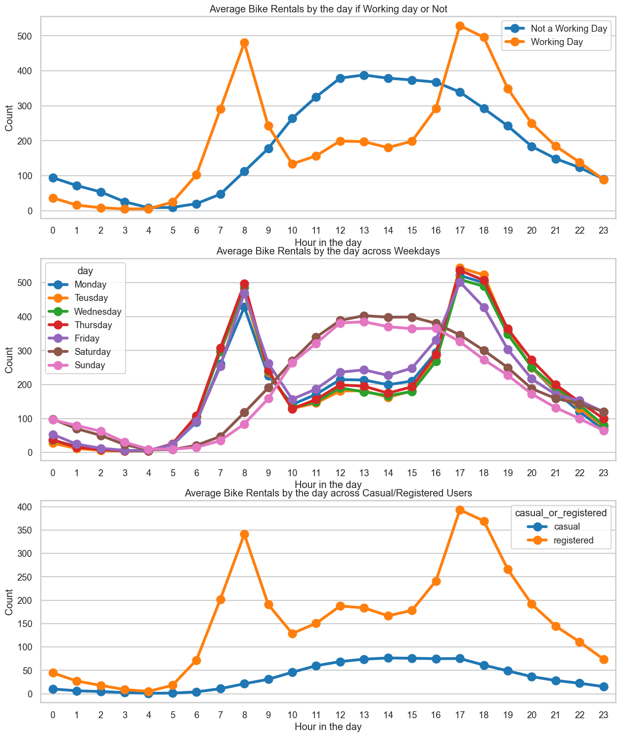

월별 분포

월별로 자전거 평균 대여수를 확인한다.

# Average Monthly Count Distribution plot
f, axes = plt.subplots(nrows=1, ncols=1, figsize=(15, 6))
group_month = pd.DataFrame(train_df.groupby(['month', 'workingday'])['count'].mean()).reset_index()
sns.barplot(data=group_month, x='month', y='count', hue='workingday', ax=axes)
axes.set(xlabel='Month', ylabel='Count', title='Average bike rentals per Month')
handles, _ = axes.get_legend_handles_labels()
axes.legend(handles, ['Not a Working Day', 'Working Day'])
plt.show()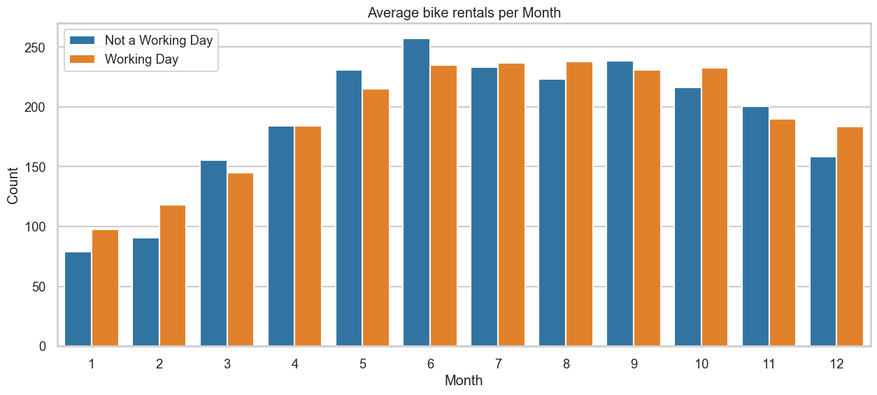

오전 8시와 오후 5시(근무시간대)에 예약이 가장 많고, 이른 아침에는 거의 없다.
두가지 패턴 관측 가능
- 근무일 : 오전 8시경에 대여가 가장 많고 오후 5시경에 또 다른 패턴 관측. 이는 일반적으로 근무일인 월-금에 출근하는 근무 지역 자전거 대여가 가장 많을 것임
- 비근무일 : 하루 종일 대여가 거의 일정하며 정오경에 가장 많은 패턴 관측. 일반적으로 낮 동안 자전거를 균일하게 대여/반납하고 비근무일인 토/일에 도시를 관광하는 관광객들이 많을 것임
가을(7-9월)과 여름(4-6월) 시즌에 자전거 대여가 많음

mydata_w = train_df[train_df.workingday==1]
mydata_nw = train_df[train_df.workingday==0]

fig = plt.figure(figsize=(18, 8))
# Working Day
axes = fig.add_subplot(1, 2, 1)
f = axes.scatter(mydata_w.hour, mydata_w['count'], c=mydata_w.temp, cmap = 'RdBu')
axes.set(xticks = range(24), xlabel='Hours in day', ylabel='Count', title='Working Day: Count vs. Day Hour with Temperature Gradient')
cbar = plt.colorbar(f)
cbar.set_label('Temperature in degree C')

# Non Working Day
axes = fig.add_subplot(1, 2, 2)
f = axes.scatter(mydata_nw.hour, mydata_nw['count'], c=mydata_nw.temp, cmap = 'RdBu')
axes.set(xticks = range(24), xlabel='Hours in day', ylabel='Count', title='Non Working Day: Count vs. Day Hour with Temperature Gradient')
cbar = plt.colorbar(f)
cbar.set_label('Temperature in degree C')

plt.show()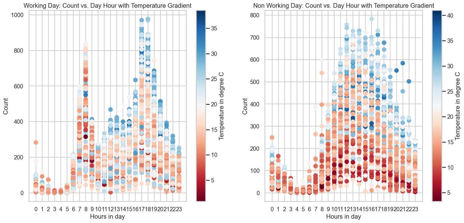

일반적으로 더 많은 사람들이 중간에서 높은 온도에서 자전거를 타는 것을 선호하는 경향. 그러나 온도가 너무 높으면 감소.

이상치 분석

날씨

폭설/비 기록이 있는 날을 어떻게 처리해야할지 알아보자. 불필요 혹은 이상치 값을 식별하고 트어떻게 처리해야 할지 결정해보자.

# Ensure the 'datetime' column is in datetime format
train_df['datetime'] = pd.to_datetime(train_df['datetime'])

# Set 'datetime' as the index
train_df.set_index('datetime', inplace=True)

# Extract heavy weather data
heavy_weather_data = train_df.loc[train_df['weather'] == 'Heavy Snow/Rain', :]
print(heavy_weather_data.index)

# Slice data for the specified datetime range
time_filtered_data = train_df['2012-01-09 08:00':'2012-01-09 20:00']

# Display the sliced data
print(time_filtered_data)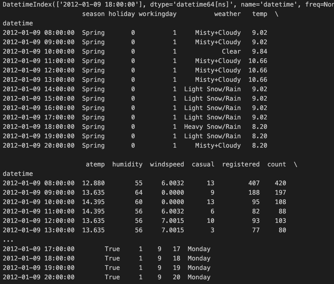

heavy_weather_data = train_df.loc[train_df['weather']=='Heavy Snow/Rain', :]
print(heavy_weather_data.index)
train_df['2012-01-09 08:00' : '2012-01-09 20:00']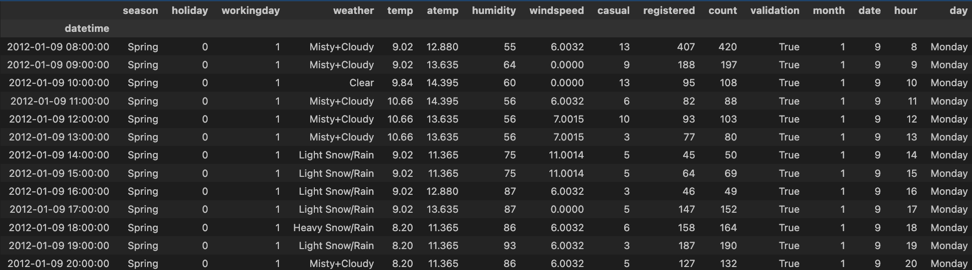

오후 6시에 날씨가 실제로 나쁜거 같다. 오전 10시에는 밝고 화창했지만 하루가 끝나갈 무렵에는 점점 더 나빠졌다. (weather = Misty->Light Snow->Heavy Snow)
Heavy Snow/Rain 는 한 번만 발생하므로 Light Snow/Rain 라벨로 바꾼다.

Z-score > 4 pruning

Z-score 이 4 표준편차 이상 떨어진 데이터를 확인한다.

# Function to calculate zscore
def zscore(series): 
    return (series-series.mean())/series.std()

train_df['count_zscore'] = train_df.groupby(['hour', 'workingday'])['count'].transform(zscore)
outlier_idx = np.abs(train_df['count_zscore'])>4
outlier_data = train_df.loc[outlier_idx, :]
print('Shape of the outlier data entries: ', outlier_data.shape)
outlier_data

Shape of the outlier data entries: (15, 17)
모든 이상치는 대부분 이른 아침이나 늦은 밤에 발생한다. 이러한 이상치를 제거해보자. 늦은 밤에는 파티가 있지 않을까?

# Removing outliers from mydata
traindata_without_outliers = train_df.loc[~outlier_idx, :]
print('Shape of data before outliner pruning: ', train_df.shape)
print('Shape of data after outlier pruning: ', traindata_without_outliers.shape)

Shape of data before outliner pruning: (10886, 17)
Shape of data after outlier pruning: (10871, 17)

# Dropping the zscore column
mydata_without_outliers = traindata_without_outliers.drop('count_zscore', axis=1)
mydata_without_outliers.head(n=3)

상관관계 분석

회귀 플롯 vs 온도,습도 및 풍속

seaborn 을 사용하여 온도, 습도, 풍속에 대한 회귀 플롯을 보자

# Regression Plots with respect to Temperature, Humidity and Windspeed
fig = plt.figure(figsize=(18, 8))
axes = fig.add_subplot(1, 3, 1)
sns.regplot(data=traindata_without_outliers, x='temp', y='count',ax=axes)
axes.set(title='Reg Plot for Temperature vs. Count')
axes = fig.add_subplot(1, 3, 2)
sns.regplot(data=traindata_without_outliers, x='humidity', y='count',ax=axes, color='r')
axes.set(title='Reg Plot for Humidity vs. Count')
axes = fig.add_subplot(1, 3, 3)
sns.regplot(data=traindata_without_outliers, x='windspeed', y='count',ax=axes, color='g')
axes.set(title='Reg Plot for Windspeed vs. Count')
plt.show()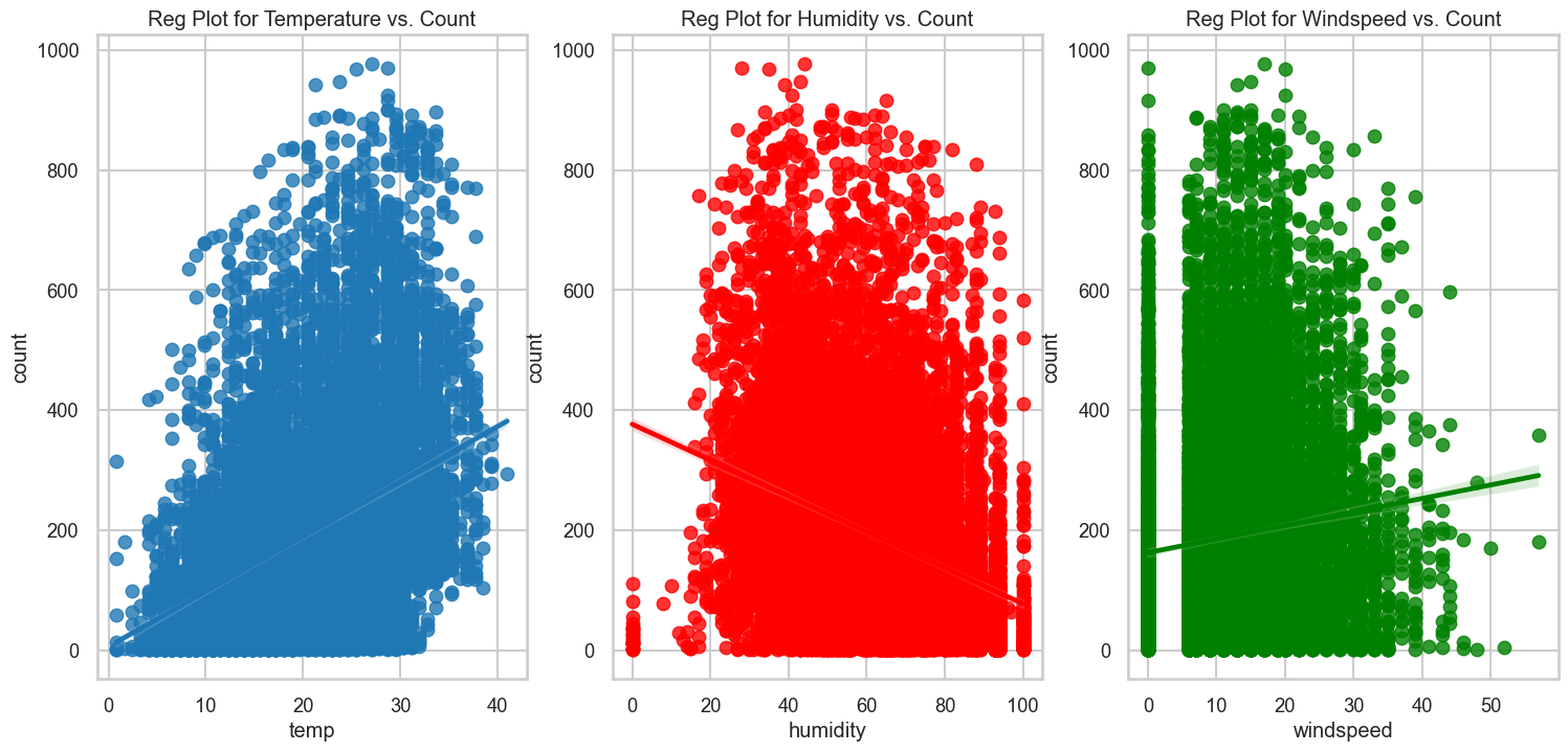

온도와 풍속과 카운트의 양의 상관관계
습도와는 음의 상관관계

히트맵

모든 수치형 데이터를 통해 자전거 대여와 다른 수치 데이터의 상관관계를 확인해보자.

# Select only numeric columns for the correlation matrix
numeric_data = traindata_without_outliers.select_dtypes(include=[np.number])

# Calculate the correlation matrix
corr_matrix = numeric_data.corr()

# Create a mask for the upper triangle
mask = np.triu(np.ones_like(corr_matrix, dtype=bool))

# Plot the heatmap
fig = plt.figure(figsize=(10, 10))
sns.heatmap(corr_matrix, mask=mask, annot=True, cbar=True, vmax=0.8, vmin=-0.8, cmap='RdYlGn')
plt.title("Heatmap of Numeric Features")
plt.show()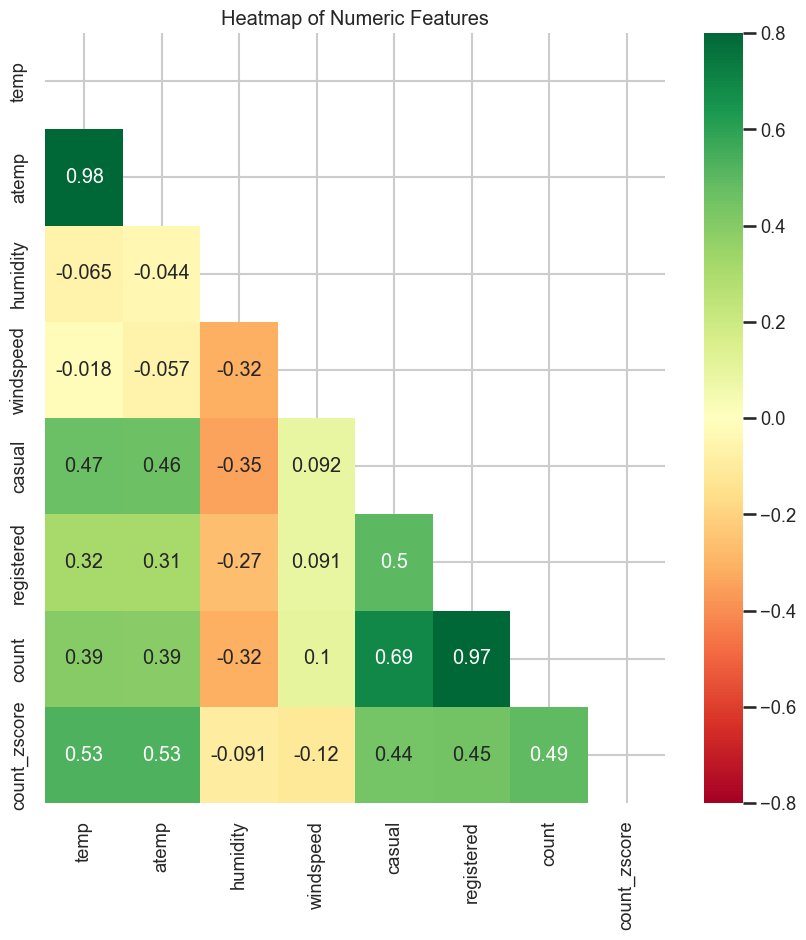

온도(실제 온도)와 온도(체감 온도)는 예상대로 높은 상관관계가 있음
count는 casual과 registered 높은 상관관계
count와 온도간의 양의 상관관계
습도와 온도는 상관관계 안큼
count는 풍속에 대한 의존석 약함

핏처 엔지니어링 - 2

많은 범주형 데이터에서 관련되고 중요한 범주형 데이터를 binary vector 컬럼으로 변환. 추후 필요하지 않은 모든 열(중복, 낮은 상관성)은 삭제
컬럼변환
- 계절 : 월과 열은 계절과 직접 매핑된다
  - 겨울(1-3월), 여름(4-6월), 가을(7-9월), 봄(10-12월)
- Holiday 와 day : 평일이며 휴일이 아니다. 근무일 중이고 근무일이 아닌 두 가지 종류의 자전거 대여 행동이 있다는 것을 알았으므로 근무일 열만 유지하고 day 와 holiday 컬럼을 삭제한다.
- 날씨 : 날씨 열을 weather_1, weather_2 and weather 3

# Using numbers to represent categorical data to transform the categorical columns
season_inv_dict = {'Spring':1, 'Summer':2, 'Fall':3, 'Winter':4}
weather_inv_dict = {'Clear':1, 'Misty+Cloudy':2, 'Light Snow/Rain':3, 'Heavy Snow/Rain':4}
day_inv_dict = {'Monday':0, 'Teusday':1, 'Wednesday':2, 'Thursday':3, 'Friday':4, 'Saturday':5, 'Sunday':6}

mydata_without_outliers['season'] = mydata_without_outliers['season'].map(season_inv_dict)
mydata_without_outliers['weather'] = mydata_without_outliers['weather'].map(weather_inv_dict)
mydata_without_outliers['day'] = mydata_without_outliers['day'].map(day_inv_dict)

test_df['season'] = test_df['season'].map(season_inv_dict)
test_df['weather'] = test_df['weather'].map(weather_inv_dict)
test_df['day'] = test_df['day'].map(day_inv_dict)

# Dropping columns from the provided data set that are either highly correlated with the existing columns: 
# season with month, holiday and day with workingday, temp with atemp
# or poorly correlated with the target column: windspeed and date
drop_columns_1 = ['season', 'holiday', 'atemp', 'windspeed', 'date', 'day']
mydata_without_outliers = mydata_without_outliers.drop(drop_columns_1, axis=1)
testdata = test_df.drop(drop_columns_1, axis=1)
mydata_without_outliers.head(n=3)

카테고리에서 바이너리 컬럼으로 변환

# Transforming all the categorical columns into binary columns
month=pd.get_dummies(mydata_without_outliers['month'], prefix='month')
weather=pd.get_dummies(mydata_without_outliers['weather'], prefix='weather')
hour=pd.get_dummies(mydata_without_outliers['hour'], prefix='hour')
mydata_train=pd.concat([mydata_without_outliers, weather, month, hour],axis=1)

month=pd.get_dummies(testdata['month'], prefix='month')
weather=pd.get_dummies(testdata['weather'], prefix='weather')
hour=pd.get_dummies(testdata['hour'], prefix='hour')
mydata_test=pd.concat([testdata, weather, month, hour],axis=1)

mydata_train.columns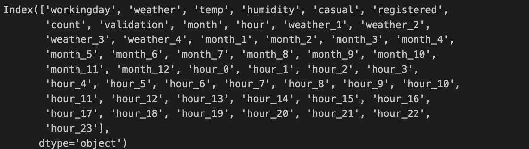

열과 마지막 binary vector 컬럼 삭제(완전히 상관관계가 있고 다른 열의 함수로 표현될 수 있음)

# Dropping columns and the last binary vector column 
drop_columns_2 = ['weather', 'month', 'hour', 'weather_3', 'month_12', 'hour_23']

mydata_train = mydata_train.drop(drop_columns_2+['casual', 'registered'], axis=1)
mydata_test = mydata_test.drop(drop_columns_2, axis=1)
mydata_without_outliers = mydata_without_outliers.drop(['casual', 'registered'], axis=1)

mydata_train.columns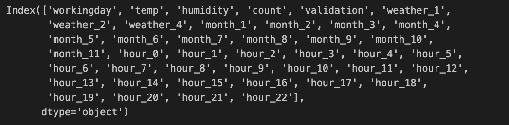

🤖 모델링

자전거 대여 추세는 근무일과 비근무일 사이에 상당히 다르기 때문에, 우리는 이 문제를 해결하기 위해 다음과 같은 두가지 방법을 시도한다.
- 두 개의 모델을 사용한다. 하나는 근무일용, 하나는 비근무일용
- 근무일을 핏처 하나로 사용

데이터 분할(Train/Validation/Test)

매달 1일부터 19일까지는 학습, 20일부터 말일까지는 테스트셋으로 설정한다.
Training set, model_train
- 매월 1일부터 15일까지 데이터가 포함
- 모델 학습을 위함
Testing set, model_test
- 매월 16일부터 19일까지의 데이터가 포함
- 모델 테스트하는데 사용
count가 제공되지 않은 최종 테스트 데이터는 20일부터 말일까지만 존재.

model_train, model_test = mydata_train[mydata_train.index.day<15], mydata_train[mydata_train.index.day>=15]
model_train2, model_test2 = mydata_without_outliers[mydata_without_outliers.index.day<15], mydata_without_outliers[mydata_without_outliers.index.day>=15]

# Separating out the working an non-working data from the training set 
model_train_w = model_train[model_train['workingday']==1]
model_train_nw = model_train[model_train['workingday']==0]
model_train2_w = model_train2[model_train2['workingday']==1]
model_train2_nw = model_train2[model_train2['workingday']==0]

model_test_w = model_test[model_test['workingday']==1]
model_test_nw = model_test[model_test['workingday']==0]
model_test2_w = model_test2[model_test2['workingday']==1]
model_test2_nw = model_test2[model_test2['workingday']==0]

# Dropping workingday column 
model_train_w = model_train_w.drop('workingday', axis=1)
model_train_nw = model_train_nw.drop('workingday', axis=1)
model_train2_w = model_train2_w.drop('workingday', axis=1)
model_train2_nw = model_train2_nw.drop('workingday', axis=1)

model_test_w = model_test_w.drop('workingday', axis=1)
model_test_nw = model_test_nw.drop('workingday', axis=1)
model_test2_w = model_test2_w.drop('workingday', axis=1)
model_test2_nw = model_test2_nw.drop('workingday', axis=1)

# Contains Binary Vector Form of features (Obtained from OneHotEncoder transformed categorical feature)
X, X_w, X_nw = model_train.drop('count', axis=1), model_train_w.drop('count', axis=1), model_train_nw.drop('count', axis=1)
y, y_w, y_nw = model_train['count'], model_train_w['count'], model_train_nw['count']
logy, logy_w, logy_nw = np.log1p(y), np.log1p(y_w), np.log1p(y_nw)

Xtest, Xtest_w, Xtest_nw = model_test.drop('count', axis=1), model_test_w.drop('count', axis=1), model_test_nw.drop('count', axis=1)
ytest, ytest_w, ytest_nw = model_test['count'], model_test_w['count'], model_test_nw['count']
logytest, logytest_w, logytest_nw = np.log1p(y), np.log1p(y_w), np.log1p(y_nw)

# Contains Categorical features instead of the Binary Vector Form
X2, X2_w, X2_nw = model_train2.drop('count', axis=1), model_train2_w.drop('count', axis=1), model_train2_nw.drop('count', axis=1)
y2, y2_w, y2_nw = model_train2['count'], model_train2_w['count'], model_train2_nw['count']
logy2, logy2_w, logy2_nw = np.log1p(y2), np.log1p(y2_w), np.log1p(y2_nw)

Xtest2, Xtest2_w, Xtest2_nw = model_test2.drop('count', axis=1), model_test2_w.drop('count', axis=1), model_test2_nw.drop('count', axis=1)
ytest2, ytest2_w, ytest2_nw = model_test2['count'], model_test2_w['count'], model_test2_nw['count']
logytest2, logytest2_w, logytest2_nw = np.log1p(y), np.log1p(y_w), np.log1p(y_nw)

# Data Frame to store all the RMSLE scores for various algorithms
algo_score = pd.DataFrame()
algo_score.index.name = 'Modelling Algo'
algo_score['Train RMSLE (Working Day)'] = None
algo_score['Train RMSLE (Non Working Day)'] = None
algo_score['Train RMSLE (Average)'] = None
algo_score['Test RMSLE (Working Day)'] = None
algo_score['Test RMSLE (Non Working Day)'] = None
algo_score['Test RMSLE (Average)'] = None
algo_score['Validation RMSLE (Working Day)'] = None
algo_score['Validation RMSLE (Non Working Day)'] = None
algo_score['Validation RMSLE (Average)'] = None
algo_score['Hyperparameters-Working'] = None
algo_score['Hyperparameters-Non Working'] = None
algo_score['Training+Test Time (sec)'] = None
cv_time = []

# Data Frame for second level of prediction. Collect the predicted y values for training and test set of data
ypred_train = pd.DataFrame(index = X.index)
ypred_test = pd.DataFrame(index = Xtest.index)
ypred_train['count'], ypred_test['count'] = y, ytest

함수 정의

모든 모델에 대해 호출할 몇 가지 함수를 정의해보자.
rmsle 와 rmsle.log

from sklearn.metrics import make_scorer

# Metric used to measure the model (Root Mean Square Log Error)
def rmsle(y_actual, y_pred):
    log1 = np.nan_to_num(np.array([np.log1p(v) for v in y_pred]))
    log2 = np.nan_to_num(np.array([np.log1p(v) for v in y_actual]))
    calc = (log1 - log2) ** 2
    return np.sqrt(np.mean(calc))

# RMSLE function with inputs in log form. Used for CrossValidation scoring
def rmsle_log(logy_actual, logy_pred):
    calc = (logy_actual - logy_pred) ** 2
    return np.sqrt(np.mean(calc))
rmsle_cv = make_scorer(rmsle_log, greater_is_better=False)

plot_true vs _pred : 특정 시간 간격에 대한 True 및 예측 카운트 값을 플로팅하는데 사용

# Plots True vs. Predictied count values in a particular time interval
def plot_true_vs_pred (y_w_actual, y_nw_actual, y_w_pred, y_nw_pred, algo, t_from, t_to):
    fig = plt.figure(figsize=(18, 16))
    
    # Working day plot
    axes = fig.add_subplot(2, 1, 1)
    axes.plot(y_w_actual[t_from:t_to], label='Actual', marker='.', markersize=15)
    axes.plot(y_w_pred[t_from:t_to], label='Predicted', marker='.', markersize=15)
    axes.set(xlabel='Time', ylabel='Count', title='{0} Model for Working Day: Count between time {1} and {2}'.format(algo, t_from, t_to))
    axes.legend()

    # Non working day plot
    axes = fig.add_subplot(2, 1, 2)
    axes.plot(y_nw_actual[t_from:t_to], label='Actual', marker='.', markersize=15)
    axes.plot(y_nw_pred[t_from:t_to], label='Predicted', marker='.', markersize=15)
    axes.set(xlabel='Time', ylabel='Count', title='{0} Model for Non Working Day: Count between time {1} and {2}'.format(algo, t_from, t_to))
    axes.legend()
    plt.show()

model_fit : 다양한 모델을 시도하여 어떤 모델이 가장 잘 작동하는지 알아낼 것이므로, 학습 데이터에 적합하고 테스트 데이터에 대해 예측하고 필요한 메트릭을 반환하는 적합 및 예측 함수를 사용자 지정.
두 가지 경우 중 하나에 대해 학습 및 테스트 데이터를 적합/예측 가능
- 근무일과 비근무일
- 근무일과 비근무일을 합친 것
결과
- 학습을 위한 rmsle, 근무일, 비근무일 및 합친 것에 대한 테스트 데이터
- 학습을 위한 예측된 y, 근무/비근무 또는 합친 것에 대한 테스트

def cross_val(model_w, X_in_w, y_in_w, model_nw=None, X_in_nw=None, y_in_nw=None, cv=5):
    y_val_pred_w = pd.Series(index=y_in_w.index)
    y_val_pred_nw = None if model_nw == None else pd.Series(index=y_in_nw.index)
    for idx in range(cv):
        from_, to_ = idx*15/cv, (idx+1)*15/cv
        
        val_idx_w = (X_in_w.index.day>from_) & (X_in_w.index.day<=to_)
        train_idx_w = ~val_idx_w
        
        X_idx_w, y_idx_w, X_val_idx_w = X_in_w[train_idx_w], y_in_w[train_idx_w], X_in_w[val_idx_w]
        model_w.fit(X_idx_w, np.log1p(y_idx_w))
        logy_val_pred_idx_w = model_w.predict(X_val_idx_w)
        y_val_pred_w[val_idx_w] = np.expm1(logy_val_pred_idx_w)
        
        if model_nw is not None:
            val_idx_nw = (X_in_nw.index.day>from_) & (X_in_nw.index.day<=to_)
            train_idx_nw = ~val_idx_nw
            
            X_idx_nw, y_idx_nw, X_val_idx_nw = X_in_nw[train_idx_nw], y_in_nw[train_idx_nw], X_in_nw[val_idx_nw]
            model_nw.fit(X_idx_nw, np.log1p(y_idx_nw))
            logy_val_pred_idx_nw = model_nw.predict(X_val_idx_nw)
            y_val_pred_nw[val_idx_nw] = np.expm1(logy_val_pred_idx_nw)
    
    if model_nw is None: 
        rmsle_avg = rmsle(y_in_w, y_val_pred_w)
        rmsle_w = rmsle(y_in_w[X_in_w.workingday==1], y_val_pred_w[X_in_w.workingday==1])
        rmsle_nw = rmsle(y_in_w[X_in_w.workingday==0], y_val_pred_w[X_in_w.workingday==0])
    else:
        rmsle_w = rmsle(y_in_w, y_val_pred_w)
        rmsle_nw = rmsle(y_in_nw, y_val_pred_nw)
        rmsle_avg = rmsle(np.concatenate([y_in_w, y_in_nw]), np.concatenate([y_val_pred_w, y_val_pred_nw]))
    
    rmsle_all = [rmsle_w, rmsle_nw, rmsle_avg]
    y_pred_all =[y_val_pred_w, y_val_pred_nw]
    return(rmsle_all, y_pred_all)

cross_val : 데이터를 cv 폴드로 분할하고, cv-1폴드에서 훈련하고, left out 폴드에서 테스트하고, 예측된 값을 저장하고 left out 폴드의 예측된 값을 저장하는데 사용. 이러한 예측합은 stacking 을 위함.
사용된 5개 폴드 : 매달 (1,3), (4,6), (7,9), (10,12), (13,15)

# Linear Regressor Ensemble for the above 3 models
def stack_model_fit (model, X_tr, X_t, y_tr, y_t):
    model.fit(X_tr, y_tr)
    y_tr_pred = model.predict(X_tr)
    y_t_pred = model.predict(X_t)
    
    [rmsle_avg_tr, rmsle_avg_t] = rmsle(y_tr, y_tr_pred), rmsle(y_t, y_t_pred)
    
    y_tr_w_pred, y_tr_nw_pred = y_tr_pred[X.workingday==1], y_tr_pred[X.workingday==0]
    y_t_w_pred, y_t_nw_pred = y_t_pred[Xtest.workingday==1], y_t_pred[Xtest.workingday==0]
    y_tr_w, y_tr_nw = y_tr[X.workingday==1], y_tr[X.workingday==0]
    y_t_w, y_t_nw = y_t[Xtest.workingday==1], y_t[Xtest.workingday==0]
    
    rmsle_w_tr, rmsle_nw_tr = rmsle(y_tr_w, y_tr_w_pred), rmsle(y_tr_nw, y_tr_nw_pred)
    rmsle_w_t, rmsle_nw_t = rmsle(y_t_w, y_t_w_pred), rmsle(y_t_nw, y_t_nw_pred)
    
    rmsle_all = [rmsle_w_tr, rmsle_nw_tr, rmsle_avg_tr, rmsle_w_t, rmsle_nw_t, rmsle_avg_t]
    y_pred_all = [y_tr_pred, y_t_pred]
    
    return(rmsle_all, y_pred_all)

stack_model_fit : 스태킹 모델을 위한 데이터 세트를 적합하고 예측하는데 사용. 입력/핏처라는 개별모델에서부터 새로운 모델을 학습시키는데 사용된다.

회귀분석

Model fit + Predict

from sklearn.linear_model import LinearRegression
lreg_w, lreg_nw = LinearRegression(), LinearRegression()

param_summary = ['', '', '']

rmsle_summary, y_predict_summary = model_fit(lreg_w, X_w, Xtest_w, y_w, ytest_w, lreg_nw, X_nw, Xtest_nw, y_nw, ytest_nw)
ypred_test.loc[Xtest.workingday==1,'LR'], ypred_test.loc[Xtest.workingday==0,'LR'] = y_predict_summary[1], y_predict_summary[3]


rmsle_val_summary, y_predict_val_summary = cross_val(lreg_w, X_w, y_w, lreg_nw, X_nw, y_nw)
ypred_train.loc[X.workingday==1,'LR'], ypred_train.loc[X.workingday==0,'LR'] = y_predict_val_summary[0], y_predict_val_summary[1]

algo_score.loc['Linear Regression'] = rmsle_summary+rmsle_val_summary+param_summary
algo_score.loc[['Linear Regression']]

과대적합이 아니다. 훈련&테스트셋이 다소 비슷 = 초기의 좋은 모델

테스트 데이터 예측

# Linear Regression Plot: True vs. Predicted for one week 
t_from, t_to = '2012-08-15', '2012-08-19'
ytest_w_predict, ytest_nw_predict = y_predict_summary[1], y_predict_summary[3]
ytest_w_predict = pd.Series(ytest_w_predict, index = ytest_w.index)
ytest_nw_predict = pd.Series(ytest_nw_predict, index = ytest_nw.index)

plot_true_vs_pred(ytest_w, ytest_nw, ytest_w_predict, ytest_nw_predict, 'Linear Regression', t_from, t_to)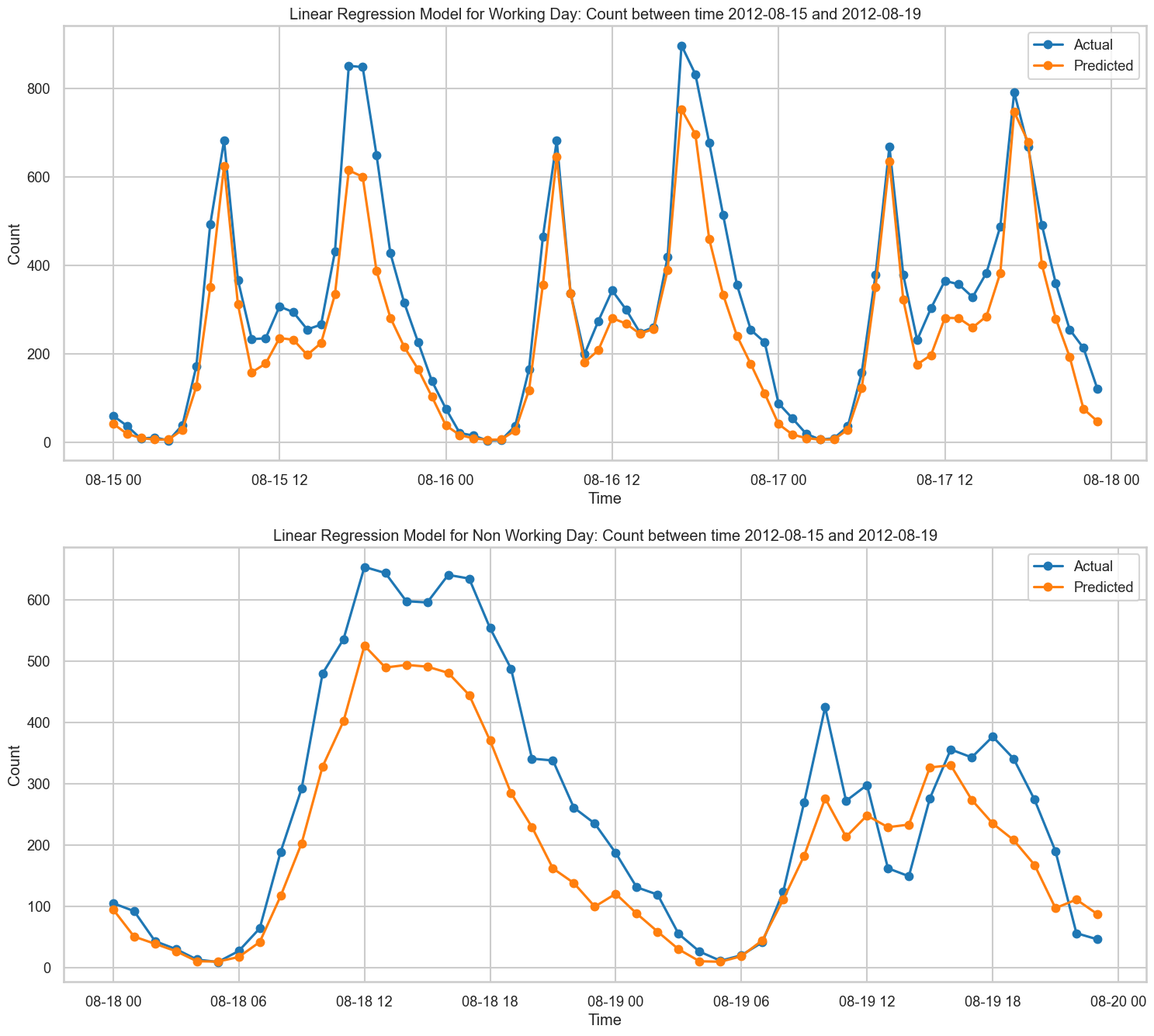

# Features and the Estimated Linear Regression Coefficients obtained for Working day and Non-working day models
df_coeff = pd.DataFrame({'features': X_w.columns, 'Lin_Coeff_Working': lreg_w.coef_, 'Lin_Coeff_Non_Working': lreg_nw.coef_})

릿지

하이퍼파라미터 튜닝

from sklearn.linear_model import Ridge
from sklearn.model_selection import GridSearchCV

# Hyperparameter Tuning
param_grid = {'alpha': [0.1, 0.2, 0.5, 1, 2, 5, 10, 20, 50, 100]}
ridge_w = GridSearchCV(Ridge(random_state=42), param_grid, cv=5, scoring=rmsle_cv)
ridge_w.fit(X_w, logy_w)
print('Best alpha for Working Day Ridge Regression Model: {}'.format(ridge_w.best_params_))
ridge_nw = GridSearchCV(Ridge(random_state=42), param_grid, cv=5, scoring=rmsle_cv)
ridge_nw.fit(X_nw, logy_nw)
print('Best alpha for Non Working Day Ridge Regression Model: {}'.format(ridge_nw.best_params_))

Best alpha for Working Day Ridge Regression Model: {'alpha': 10}
Best alpha for Non Working Day Ridge Regression Model: {'alpha': 10}

Model fit + Predict

param_summary = [ridge_w.best_params_, ridge_nw.best_params_,'']

rmsle_summary, y_predict_summary = model_fit(ridge_w, X_w, Xtest_w, y_w, ytest_w, ridge_nw, X_nw, Xtest_nw, y_nw, ytest_nw)
ypred_test.loc[Xtest.workingday==1,'Ridge'], ypred_test.loc[Xtest.workingday==0,'Ridge'] = y_predict_summary[1], y_predict_summary[3]

rmsle_val_summary, y_predict_val_summary = cross_val(ridge_w, X_w, y_w, ridge_nw, X_nw, y_nw)
ypred_train.loc[X.workingday==1,'Ridge'], ypred_train.loc[X.workingday==0,'Ridge'] = y_predict_val_summary[0], y_predict_val_summary[1]

algo_score.loc['Ridge Regression'] = rmsle_summary+rmsle_val_summary+param_summary
algo_score.loc[['Ridge Regression']]

algo_score.loc['Ridge Regression', 'Training+Test Time (sec)'] = 1.3
cv_time.append(4.64)

회귀분석과 같은 퍼포먼스

테스트 데이터 예측

# Ridge Regression Plot: True vs. Predicted for one month 
t_from, t_to = '2012-08-15', '2012-08-19'
ytest_w_predict, ytest_nw_predict = y_predict_summary[1], y_predict_summary[3]
ytest_w_predict = pd.Series(ytest_w_predict, index = ytest_w.index)
ytest_nw_predict = pd.Series(ytest_nw_predict, index = ytest_nw.index)

plot_true_vs_pred(ytest_w, ytest_nw, ytest_w_predict, ytest_nw_predict, 'Ridge Regularization Regression', t_from, t_to)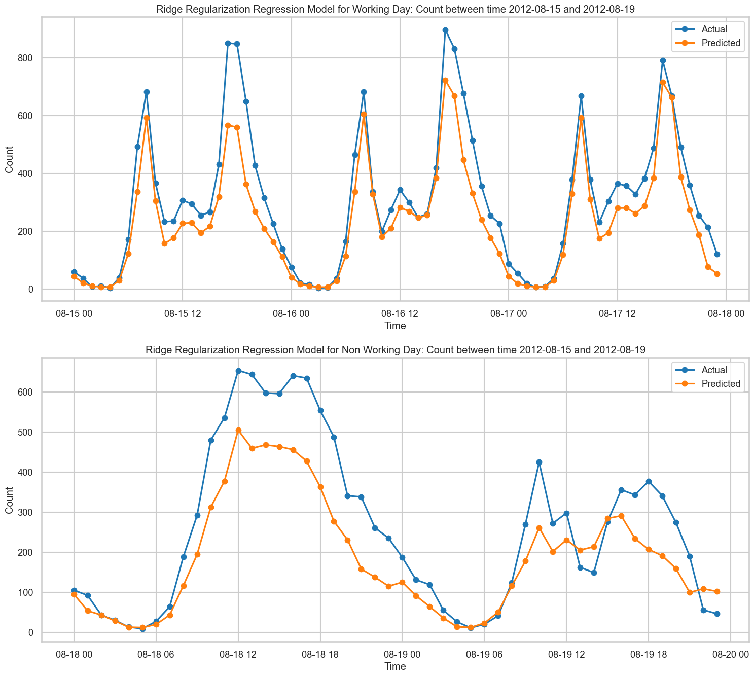

라쏘

하이퍼파라미터 튜닝

# Lasso Regression
from sklearn.linear_model import Lasso
from sklearn.model_selection import GridSearchCV

# Hyperparameter Tuning
param_grid = {'alpha': [0.1, 0.2, 0.5, 1, 2, 5, 10, 20, 50, 100]}
lasso_w = GridSearchCV(Lasso(random_state=42), param_grid, cv=5, scoring=rmsle_cv)
lasso_w.fit(X_w, logy_w)
print('Best alpha for Working Day Lasso Regression Model: {}'.format(lasso_w.best_params_))

lasso_nw = GridSearchCV(Lasso(random_state=42), param_grid, cv=5, scoring=rmsle_cv)
lasso_nw.fit(X_nw, logy_nw)
print('Best alpha for Non Working Day Lasso Regression Model: {}'.format(lasso_nw.best_params_))

Best alpha for Working Day Lasso Regression Model: {'alpha': 0.1}
Best alpha for Non Working Day Lasso Regression Model: {'alpha': 0.5}

Model fit + Predict

param_summary = [lasso_w.best_params_, lasso_nw.best_params_,'']

rmsle_summary, y_predict_summary = model_fit(lasso_w, X_w, Xtest_w, y_w, ytest_w, lasso_nw, X_nw, Xtest_nw, y_nw, ytest_nw)
ypred_test.loc[Xtest.workingday==1,'Lasso'], ypred_test.loc[Xtest.workingday==0,'Lasso'] = y_predict_summary[1], y_predict_summary[3]

rmsle_val_summary, y_predict_val_summary = cross_val(lasso_w, X_w, y_w, lasso_nw, X_nw, y_nw)
ypred_train.loc[X.workingday==1,'Lasso'], ypred_train.loc[X.workingday==0,'Lasso'] = y_predict_val_summary[0], y_predict_val_summary[1]

algo_score.loc['Lasso Regression'] = rmsle_summary+rmsle_val_summary+param_summary
algo_score.loc[['Lasso Regression']]

algo_score.loc['Lasso Regression', 'Training+Test Time (sec)'] = 1.3
cv_time.append(4.57)

RMSLE 값이 1 이상이기에 굉장히 좋지 않음

테스트 데이터 예측

# Lasso Regression Plot: True vs. Predicted for one month 
t_from, t_to = '2012-08-15', '2012-08-19'
ytest_w_predict, ytest_nw_predict = y_predict_summary[1], y_predict_summary[3]
ytest_w_predict = pd.Series(ytest_w_predict, index = ytest_w.index)
ytest_nw_predict = pd.Series(ytest_nw_predict, index = ytest_nw.index)

plot_true_vs_pred(ytest_w, ytest_nw, ytest_w_predict, ytest_nw_predict, 'Lasso Regularization Regression', t_from, t_to)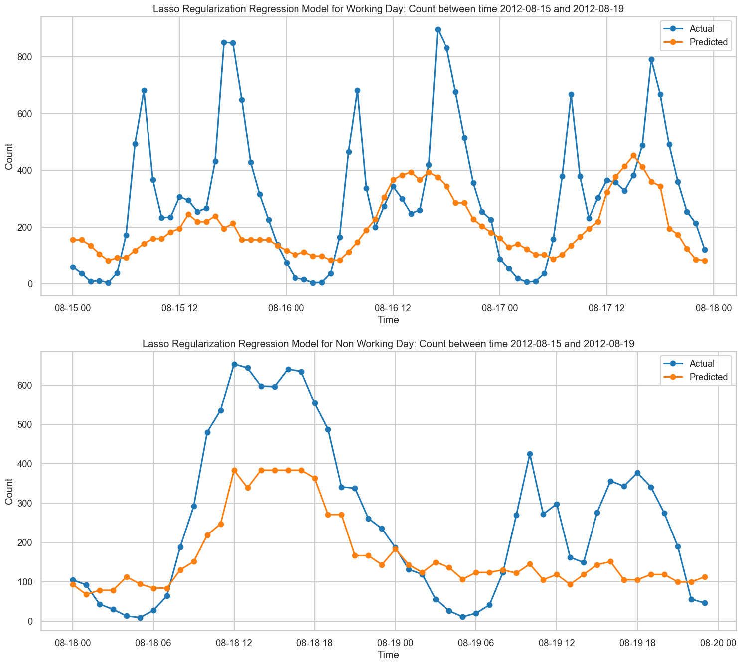

회귀분석 vs 릿지 vs 라쏘 계수비교

# Add Ridge and Lasso coefficients for working day models
df_coeff['Ridge_Coeff_Working'] = ridge_w.best_estimator_.coef_
df_coeff['Lasso_Coeff_Working'] = lasso_w.best_estimator_.coef_

# Add Ridge and Lasso coefficients for non-working day models
df_coeff['Ridge_Coeff_Non_Working'] = ridge_nw.best_estimator_.coef_
df_coeff['Lasso_Coeff_Non_Working'] = lasso_nw.best_estimator_.coef_

import matplotlib.pyplot as plt

# Plotting the feature coefficients for Linear, Ridge, and Lasso Regression Models
fig = plt.figure(figsize=(18, 18))

# Working day plot
axes = fig.add_subplot(2, 1, 1)
axes.plot(df_coeff['Lin_Coeff_Working'], label='Linear Regression', marker='.', markersize=15)
axes.plot(df_coeff['Ridge_Coeff_Working'], label='Ridge Regression, alpha={}'.format(ridge_w.best_params_['alpha']), marker='.', markersize=15)
axes.plot(df_coeff['Lasso_Coeff_Working'], label='Lasso Regression, alpha={}'.format(lasso_w.best_params_['alpha']), marker='.', markersize=15)
axes.axvline(2-0.5, c='k', ls='--')
axes.axvline(4-0.5,  c='k', ls='--')
axes.axvline(15-0.5,  c='k', ls='--')
plt.xticks(range(len(df_coeff['Lin_Coeff_Working'])), df_coeff['features'], rotation=90)
axes.set(ylabel='Estimated Regression Coefficients', title='Coefficients for Working Day Model')
axes.set(xlim=[-1, len(df_coeff['Lin_Coeff_Working'])])
axes.legend()

# Non-working day plot
axes = fig.add_subplot(2, 1, 2)
axes.plot(df_coeff['Lin_Coeff_Non_Working'], label='Linear Regression', marker='.', markersize=15)
axes.plot(df_coeff['Ridge_Coeff_Non_Working'], label='Ridge Regression, alpha={}'.format(ridge_nw.best_params_['alpha']), marker='.', markersize=15)
axes.plot(df_coeff['Lasso_Coeff_Non_Working'], label='Lasso Regression, alpha={}'.format(lasso_nw.best_params_['alpha']), marker='.', markersize=15)
axes.axvline(2-0.5, c='k', ls='--')
axes.axvline(4-0.5,  c='k', ls='--')
axes.axvline(15-0.5,  c='k', ls='--')
plt.xticks(range(len(df_coeff['Lin_Coeff_Working'])), df_coeff['features'], rotation=90)
axes.set(ylabel='Estimated Regression Coefficients', title='Coefficients for Non-Working Day Model')
axes.set(xlim=[-1, len(df_coeff['Lin_Coeff_Working'])])
axes.legend()

plt.show()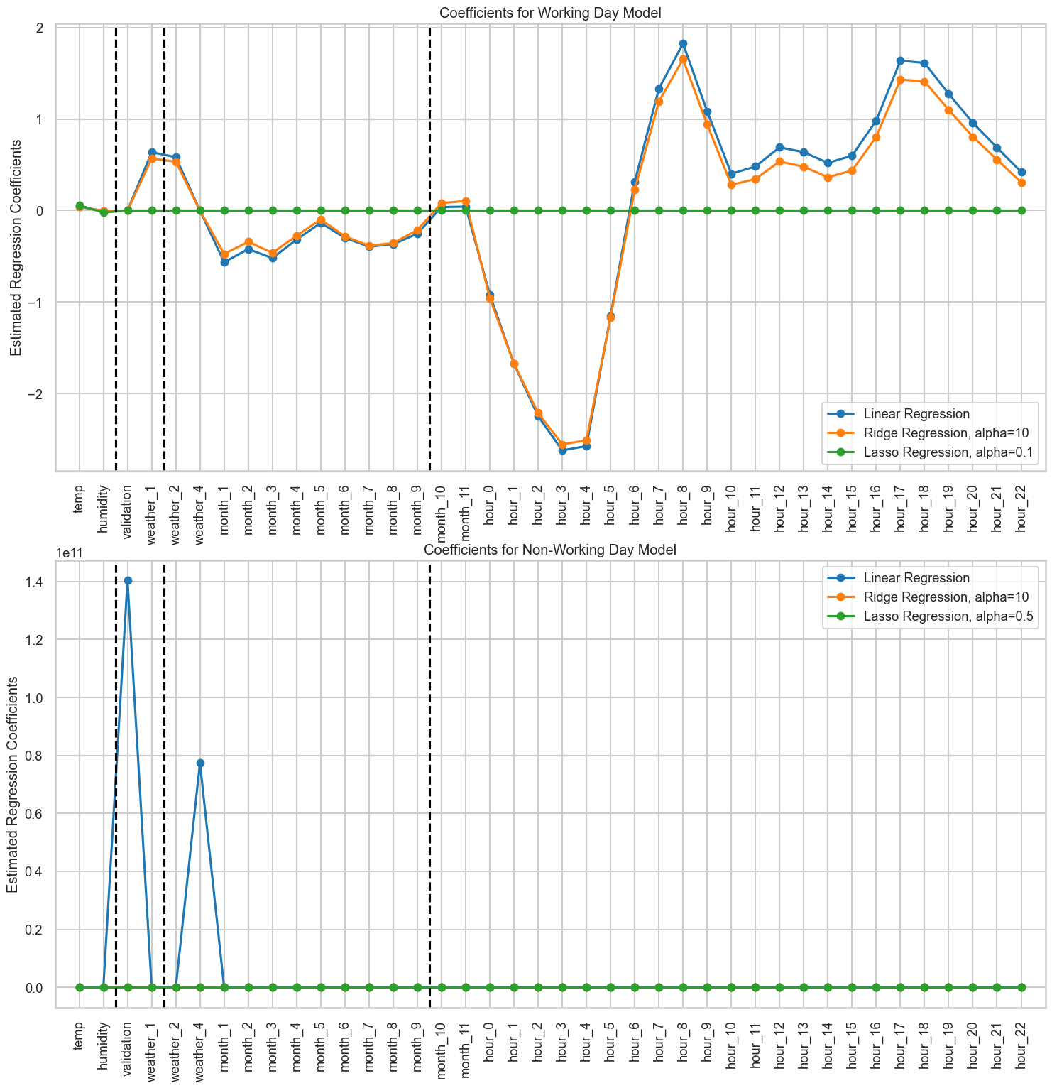

앙상블 - 랜덤 포레스트

싱글 모델(근무일, 비근무일) + 카테고리 컬럼

랜덤 포레스트 회귀는 의사결정 트리를 기반으로 예측하기 때문에 시간, 월, 근무일 및 비근무일을 포함한 범주형 피처를 처리할 수 있다. 먼저 변환된 핏처 + 근무/비근무에 대한 2개의 모델을 사용하는 대신 핏처를 만든 모델에 포함시켜 시작한다.

X2.head(n=3)

하이퍼 파라미터 튜닝

n_estimators 를 나머지 매개변수의 기본값을 사용하여 얻는다.
최적의 n_estimators를 사용하여 max_features를 얻는다(조정)
최적의 n_estimators 와 max_features를 사용하여 최적의 min_samples_leaf를 얻는다.(조정)
n_estimators,max_features, min_samples_leaf 를 사용하여 최적의 max_depth를 얻는다.
지금까지 얻은 변수들을 통해 min_samples_split을 조정한다.

## Random Forest Regression Hyperparameter tuning using Grid Search to obtain the best parameters. 
## Commented it out since it takes a lot of time to run. Using the best parameters obtained via the below search
from sklearn.ensemble import RandomForestRegressor
from sklearn.model_selection import GridSearchCV

#param_grid = {'n_estimators': [50, 100, 200, 500, 1000, 2000, 5000]}
#rf_main = GridSearchCV(RandomForestRegressor(random_state=42), param_grid, cv=5, scoring=rmsle_cv)
#rf_main.fit(X2, logy2)

#param_grid = {'n_estimators': [500], 'max_features':['auto', 'sqrt', 'log2']}
#rf_main = GridSearchCV(RandomForestRegressor(random_state=42), param_grid, cv=5, scoring=rmsle_cv)
#rf_main.fit(X2, logy2)

#param_grid = {'n_estimators': [500], 'max_features':['auto'], 'min_samples_leaf':[1, 3, 7, 10, 20, 50]}
#rf_main = GridSearchCV(RandomForestRegressor(random_state=42), param_grid, cv=5, scoring=rmsle_cv)
#rf_main.fit(X2, logy2)

#param_grid = {'n_estimators': [500], 'max_features':['auto'], 'min_samples_leaf':[7], 'max_depth':[5, 8, 10, 20, 30, 40, 50, 70]}
#rf_main = GridSearchCV(RandomForestRegressor(random_state=42), param_grid, cv=5, scoring=rmsle_cv)
#rf_main.fit(X2, logy2)

#param_grid = {'n_estimators': [500], 'max_features':['auto'], 'min_samples_leaf':[7], 'max_depth':[10], 'min_samples_split':[0.0001, 0.001, 0.002, 0.005, 0.01]}
#rf_main = GridSearchCV(RandomForestRegressor(random_state=42), param_grid, cv=5, scoring=rmsle_cv)
#rf_main.fit(X2, logy2)

#print('Best parameters for Random Forest Regression Model: {}'.format(rf_main.best_params_))

하이퍼 파라미터 튜닝 스코어

# All the below results are obtained from the above GridSearchCV hyperparamter tuning
fig=plt.figure(figsize=(18, 12))

n_est_array = [50, 100, 200, 500, 1000, 2000, 5000]
n_est_cv_score = [-0.59522862, -0.59345376, -0.59307606, -0.59260841, -0.59292831,-0.59274538, -0.59279494]
axes=fig.add_subplot(2, 3, 1)
axes.plot(n_est_array, n_est_cv_score, marker='.')
axes.set(xlabel='n_estimators', ylabel='Mean CV Test Score', title='n_estimators vs. Score (best_n_estimator = 500)')

max_feature_array = ['auto', 'sqrt', 'log2']
max_feature_cv_score = [-0.59260841, -0.60178303, -0.60178303]
axes=fig.add_subplot(2, 3, 2)
axes.plot(range(3), max_feature_cv_score, marker='.')
plt.xticks(range(3), max_feature_array)
axes.set(xlabel='max_feature', ylabel='Mean CV Test Score', title='max_feature vs. Score (best_max_feature = auto)')

min_samples_leaf_array = [1, 3, 7, 10, 20, 50]
min_samples_leaf_cv_score = [-0.59260841, -0.58788348, -0.58764415, -0.59060404, -0.60340495,-0.63367843]
axes=fig.add_subplot(2, 3, 3)
axes.plot(min_samples_leaf_array, min_samples_leaf_cv_score, marker='.')
axes.set(xlabel='min_samples_leaf', ylabel='Mean CV Test Score', title='min_samples_leaf vs. Score (best_min_samples_leaf = 7)')

max_depth_array = [5, 8, 10, 15, 20, 30, 40, 50, 70]
max_depth_cv_score = [-0.71808668, -0.60209726, -0.58727382, -0.58785334, -0.58764068, -0.58764415, -0.58764415, -0.58764415, -0.58764415]
axes=fig.add_subplot(2, 3, 4)
axes.plot(max_depth_array, max_depth_cv_score, marker='.')
axes.set(xlabel='max_depth', ylabel='Mean CV Test Score', title='max_depth vs. Score (best_max_depth = 10)')

min_samples_split_array = [0.0001, 0.001, 0.002, 0.005, 0.01]
min_samples_split_cv_score = [-0.58727382, -0.58727382, -0.58796633, -0.59735637, -0.61832167]
axes=fig.add_subplot(2, 3, 5)
axes.plot(min_samples_split_array, min_samples_split_cv_score, marker='.')
axes.set(xlabel='min_samples_split', ylabel='Mean CV Test Score', title='min_samples_split vs. Score (best_min_samples_split = 0.0001)')

plt.show()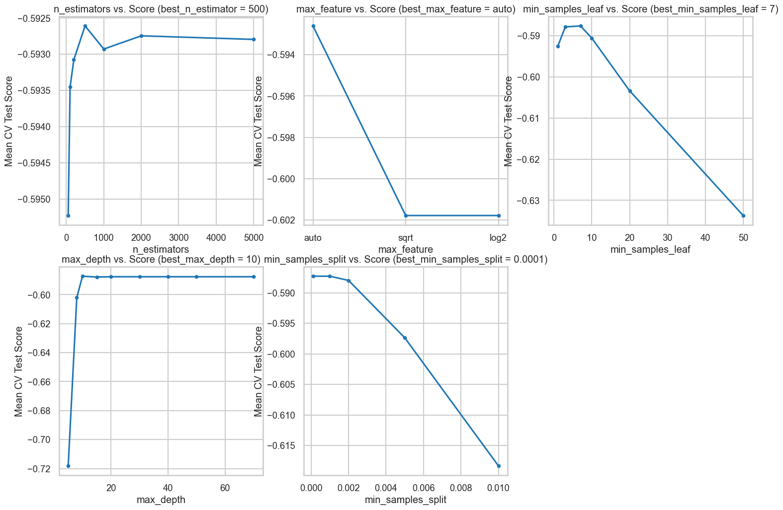

모델 동작
- 500개의 트리수와 10의 뎁스가 모델 성능을 극대화함
- 모든 특징(auto)을 각 분할에서 사용하는 것이 성능을 향상시키며, 제한적인 특징 수는 성능에 부정적인 영향을 끼침
- min_samples_leaf 와 min_samples_split ㄱ밧을 낮게 설정하면 더 세밀한 패턴을
모델의 성능을 최적화하기 위한 최적값을 설정하면 과적합 방지 및 높은 정확도 구측 가능

Model fit + Predict

from sklearn.ensemble import RandomForestRegressor

# Best parameters obtained via GridSearchCV or defined manually
best_n_estimators = 500
best_max_features = 'sqrt'  # Replace 'auto' with 'sqrt', 'log2', or a valid value
best_min_samples_leaf = 7
best_max_depth = 10

# Update param_summary to reflect the new max_features value
param_summary = [
    f'n_estimators: {best_n_estimators}, max_features: {best_max_features}, '
    f'min_samples_leaf: {best_min_samples_leaf}, max_depth: {best_max_depth}',
    f'n_estimators: {best_n_estimators}, max_features: {best_max_features}, '
    f'min_samples_leaf: {best_min_samples_leaf}, max_depth: {best_max_depth}',
    ''
]

# Initialize the RandomForestRegressor with the corrected parameter
rfa = RandomForestRegressor(
    n_estimators=best_n_estimators,
    max_features=best_max_features,
    min_samples_leaf=best_min_samples_leaf,
    max_depth=best_max_depth,
    random_state=42
)

# Fit the model using the helper function
rmsle_summary, y_predict_summary = model_fit(rfa, X2, Xtest2, y2, ytest2)

# Add predictions to the DataFrame
ypred_test['RF1'] = y_predict_summary[1]

rmsle_val_summary, y_predict_val_summary = cross_val(rfa, X2, y2)
ypred_train['RF1'] = y_predict_val_summary[0]

algo_score.loc['Random Forest-Categorical+Single'] = rmsle_summary+rmsle_val_summary+param_summary
algo_score.loc[['Random Forest-Categorical+Single']]

algo_score.loc['Random Forest-Categorical+Single', 'Training+Test Time (sec)'] = 5.48
cv_time.append(19.9)

테스트 데이터 예측

# Random Forest Regression Plot: True vs. Predicted for one month 
t_from, t_to = '2012-08-15', '2012-08-19'
y_test_predict =  pd.Series(y_predict_summary[1], index = ytest2.index) 
ytest_w_predict, ytest_nw_predict = y_test_predict[Xtest2.workingday==1], y_test_predict[Xtest2.workingday==0]
plot_true_vs_pred(ytest2_w, ytest2_nw, ytest_w_predict, ytest_nw_predict, 'Random Forest Regression', t_from, t_to)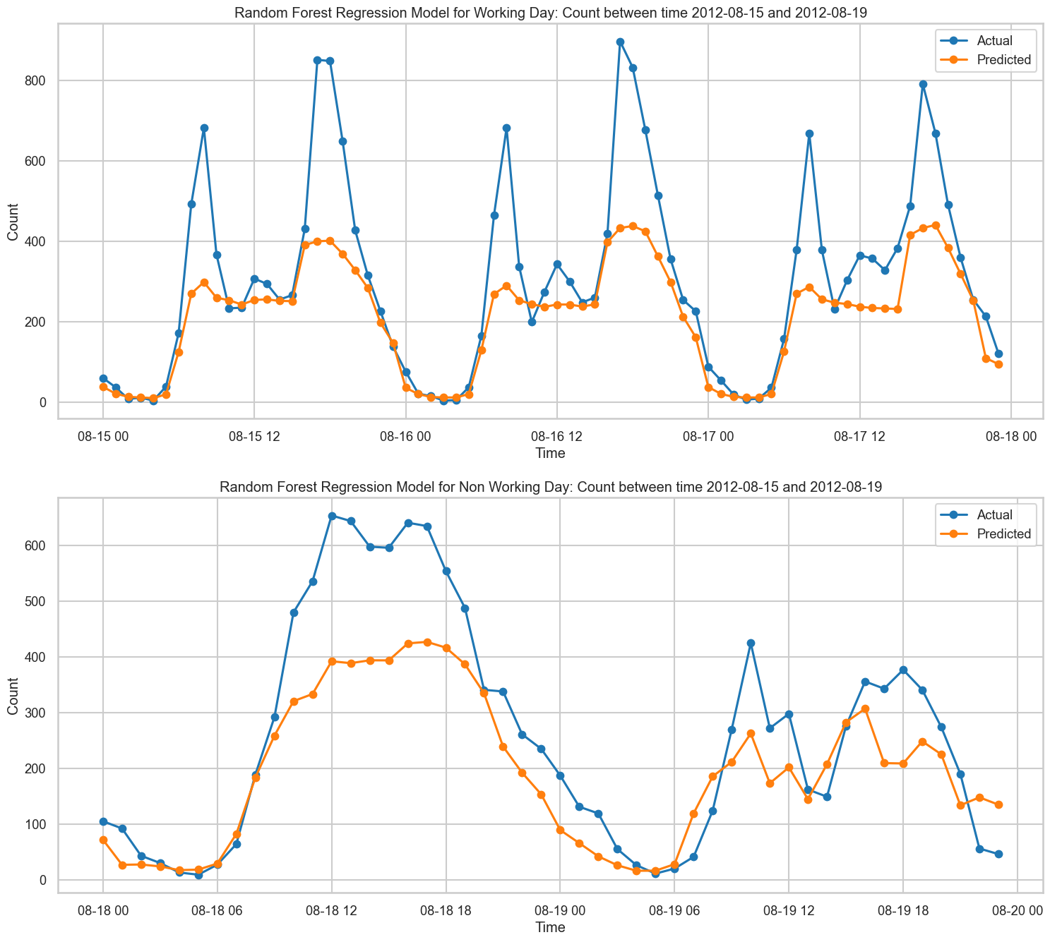

8/19 예측과 8/18 비근무일 예측 데이터에 대한 예측에 약간의 불규칙성이 있음을 알 수 있다. 이 날짜의 데이터를 살펴보고 모델 예측이 의미가 있는지 확인해보자.

Xtest2['2012-08-19 09':'2012-08-19 15']

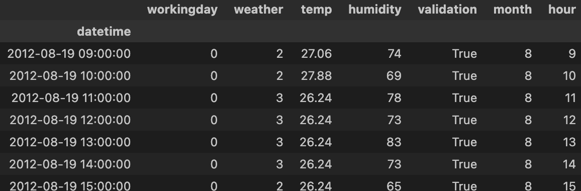
19일 11시에서 14시 사이에 날씨가 나빠지는 것을 알 수 있음. 결과적으로 모델은 그 시간대에 더 낮은 카운트 예측

Feature Importance

# Plotting the Feature Importance
fig = plt.figure(figsize=(8, 6))
axes = fig.add_subplot(1, 1, 1)
axes.plot(rfa.feature_importances_, marker='.', markersize=15)
plt.xticks(range(len(rfa.feature_importances_)), X2.columns)
axes.set(ylabel='Feature Importance', title='Feature Importance for Random Forest Regression using Categorical Data')
axes.set(xlim=[-1, len(X2.columns)], ylim=[0, 1])

plt.show()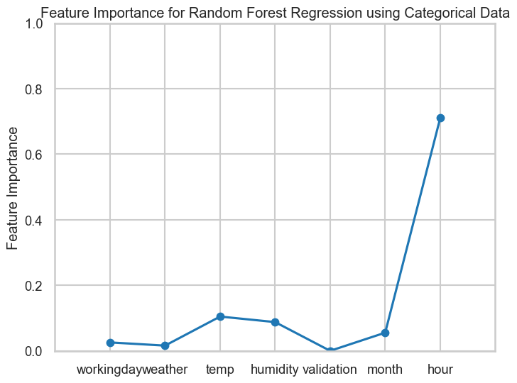

예상대로 '시간' 이 중요함. 시간에 따라 카운트 값에 급증, 감소
근무일 기능이 한계적 중요도를 가짐

🧩 문제정의

특정 시간대의 자전거 대여 패턴은 어떻게 나올까?
-> 출근시간에 자전거 대여 수요가 급증. 이는 직장인이나 학생들이 통근 및 통학 목적으로 자전거를 이용하고, 퇴근시간에는 퇴근 후 집으로 돌아가는 이동에 자전거를 활용하는 경우가 많음. 주중 저녁 및 주말 낮 시간대에는 수요가 완만하며, 여가 활동이나 레저 목적으로 이용하는 경향이 강하다.

날씨 변수와 자전거 대여 수요 간의 상관관계는 무엇인가요?
-> 기온(temp), 체감온도(atemp), 습도(humidity), 풍속(windspeed), 날씨 상태(weather)

계절별 자전거 대여 패턴의 차이는 무엇인가요?
-> 봄에는 수요가 점차 증가하는 시기. 여름에는 수요가 가장 높은 계절(적정 기온과 긴 낮 시간). 가을에는 여름과 비슷하게 높은 수치를 보이며, 날씨가 선선한 경우에 대여 활발. 겨울에는 수요가 가장 낮은 계절

주말과 평일의 자전거 대여 수요 차이는 무엇인가요?
-> 주말에는 여가 및 레저 목적의 대여가 많아지며, 수요가 낮 시간대(오전10시-오후4시)에 분포. 평일 출퇴근 시간에 집중(오전8시9시, 오후5시7시)

자전거 대여 수요를 예측하기 위해 사용할 수 있는 가장 중요한 변수는 무엇인가요?
-> 모델 분석 결과와 변수 주요도에 따르면 시간, 기온, 체감 온도, 습도, 날씨 상태, 요일 및 주말이 될 수 있다.

자전거 대여 수요 예측 모델을 구축하고, 이를 기반으로 한 운영 전략을 제안해보세요.
-> 랜덤포레스트를 이용하여 자전거 대여 수요를 예측한 결과, RMSLE를 기준으로 중요변수를 고려하여 높은 정확도를 달성했다. 시간대별 자전거 배치 최적화, 계절별 운영 계획, 날씨 기반 예측 활용, 가격 및 프로모션 전략이 있을 수 있다.

💡 가설 및 실험 설계

단순 회귀 모델과 랜덤 포레스트 성능을 비교해 더 나은 예측 모델 선택

✅ 검증

🔄 회고

성과 및 개선점

랜덤 포레스트 모델을 통한 변수별 자전거 대여 수요 예측
개선점
- 날씨 변수 한계 : 날씨 변수를 더 세분화 할 필요가 있음
- 데이터 불균형 : 특정 시간대와 계절의 데이터가 부족하여 모델의 일반화 성능에 영향을 미침
- 시간 지연 변수 추가 : 과거 대여 수요를 반영하는 시계열적 변수를 추가하여 예측 정확도를 개선할 수 있음

코드

os.path -> pathlib
지금까지 os 모듈을 사용했지만, pathlib 모듈에 더 익숙해지려 한다. 외우자!!!

# os
def read_csv(file_name):
    df = pd.read_csv(f'./interim/{file_name}.csv')
    return df
    
# Pathlib
def read_csv(file_name):
    file_path = Path('/Users/jaewon/Desktop/mission') / f"{file_name}.csv"
    df = pd.read_csv(file_path)
    return df

Jaewon Lim

이전 포스트

[경제] 금리2

다음 포스트